Transcription
Elements of Information TheoryThomas M. Cover, Joy A. ThomasCopyright 1991 John Wiley & Sons, Inc.Print ISBN 0-471-06259-6 Online ISBN 0-471-20061-1Chapter 15Information Theory andthe Stock MarketThe duality between the growth rate of wealth in the stock market andthe entropy rate of the market is striking. We explore this duality in thischapter. In particular,we shall find the competitivelyoptimalandgrowth rate optimal portfolio strategies. They are the same, just as theShannon code is optimal both competitivelyand in expected value indata compression. We shall also find the asymptotic doubling rate for anergodic stock market process.15.1THE STOCKMARKET:SOMEDEFINITIONSA stock market is represented as a vector of stocks X (X1, X,, . . . , X, 1,Xi 1 0, i 1,2, . . . ) m, where m is the number of stocks and the pricerelative Xi represents the ratio of the price at the end of the day to theprice at the beginning of the day. So typically Xi is near 1. For example,Xi 1.03 means that the ith stock went up 3% that day.Let X - F(x), where F(x) is the joint distributionof the vector of pricerelatives.b (b,, b,, . . . , b,), bi I 0, C bi 1, is an allocation ofA portfoliowealth across the stocks. Here bi is the fraction of one’s wealth investedin stock i.If one uses a portfolio b and the stock vector is X, the wealth relative(ratio of the wealth at the end of the day to the wealth at the beginningof the day) is S b’X.We wish to maximize S in some sense. But S is a random variable, sothere is controversy over the choice of the best distributionfor S. Thestandardtheory of stock marketinvestmentis based on the con459
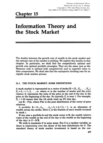
460INFORMATIONTHEORY ANDTHE STOCKMARKETsiderationof the first and second moments of S. The objective is tomaximizethe expected value of S, subject to a constrainton thevariance. Since it is easy to calculate these moments, the theory issimpler than the theory that deals wth the entire distributionof S.The mean-varianceapproach is the basis of the Sharpe-Markowitztheory of investmentin the stock market and is used by businessanalysts and others. It is illustratedin Figure 15.1. The figureillustratesthe set of achievable mean-variancepairs using variousportfolios.The set of portfolioson the boundaryof this regioncorresponds to the undominatedportfolios:these are the portfolioswhich have the highest mean for a given variance. This boundary iscalled the efficient frontier, and if one is interested only in mean andvariance, then one should operate along this boundary.Normallythe theory is simplified with the introductionof a risk-freeasset, e.g., cash or Treasury bonds, which provide a fixed interest ratewith variance 0. This stock corresponds to a point on the Y axis in thefigure. By combining the risk-free asset with various stocks, one obtainsall points below the tangent from the risk-free asset to the efficientfrontier. This line now becomes part of the efficient frontier.The concept of the efficient frontier also implies that there is a truevalue for a stock corresponding to its risk. This theory of stock prices iscalled the Capital Assets Pricing Model and is used to decide whetherthe market price for a stock is too high or too low.Looking at the mean of a random variable gives informationaboutthe long term behavior of the sum of i.i.d. versions of the randomvariable. But in the stock market, one normally reinvests every day, sothat the wealth at the end of n days is the product of factors, one foreach day of the market. The behavior of the product is determinednotby the expected value but by the expected logarithm.This leads us todefine the doubling rate as follows:Definition:The doublingrate of a stock marketportfoliob is definedasMeanSet of achievablemean -variance pairsRisk -freeasset/Figure 15.1. Sharpe-MarkowitzVariancetheory: Set of achievable mean-variancepairs.
15.1THE STOCKMARKET:SOME461DEFZNZTZONSW(b, F) 1 log btx /P(x) E(log btX) .Definition:The optimaldoublingrate W*(F)(15.1)is defined asW*(F) rnbax W(b, F),where the maximumis over all possible portfoliosDefinition:A portfolio b* thatcalled a log-optimalportfolio.The definitionTheoremof doubling15.1.1:(15.2)bi I 0, Ci bi 1.achieves the maximumrate is justifiedLet X,, X,, . . . ,X,of W(b, F) isby the followingbe i.i.d. accordingtheorem:to F(x). LetSo b*tXi(15.3)i lbe the wealth after n days using the constantThen;1ogs: w*rebalancedwith probabilityportfolio1 .b*.(15.4)Proof:(15.5) log So log b*tXii W*by the strong law of large numbers.with probabilityHence, Sz G 2”w*.We now consider some of the propertiesLemmain F.Proof:151.1:(15.6)qof the doublingrate.W(b, F) is concave in b and linear in F. W*(F) is convexThe doublingrate isW(b, F) / log btx dF(x) .Since the integralSince1,is linearin F, so is W(b, F).(15.7)
1NFORMATlON462lo& Ab, (I-THEORYANDTHE STOCKMARKETA)b,)tX 2 A log bt,X (1 - A) log bt,X 3(15.8)by the concavity of the logarithm,it follows, by taking expectations, thatW(b, F) is concave in b.Finally, to prove the convexity of W*(F) as a function of F, let Fl andF, be two distributionson the stock market and let the correspondingoptimal portfolios be b*(F,) and b*(F,) respectively. Let the log-optimalportfolio correspondingto AF, (1 - A)F, be b*( AF, (1 - A)F, ). Thenby linearity of W(b, F) with respect to F, we haveW*( AF, (1 - A)F,) W(b*( AF, (1 - A)F,), AF, (1 - A)F,) AW(b*( AF, (1 - A)&), F,) (Ix W(b*(AF,5 AW(b*(F,),since b*(F, ) maximizesLemma15.1.2:(15.9)A) (1 - AIF,), F2)F,) (1 -h)W*(b*(&), & 3 (15.10)W(b, Fl ) and b*(Fz 1 mak-nizesThe set of log-optimalportfoliosW(b, F&0forms a convex set.Proof: Let bT and bz be any two portfolios in the set of log-optimalportfolios. By the previous lemma, the convex combinationof bT and bghas a doubling rate greater than or equal to the doubling rate of bT orbg, and hence the convex combinationalso achieves the maximumdoubling rate. Hence the set of portfolios that achieves the maximumisconvex. qIn the next section, we will use these propertieslog-optimalportfolio.15.2 KUHN-TUCKERCHARACTERIZATIONLOG-OPTIMALPORTFOLIOto characterizetheOF THEThe determinationb* that achieves W*(F) is a problem of maximizationof a concave function W(b, F) over a convex set b E B. The maximummay lie on the boundary.We can use the standard Kuhn-Tuckerconditions to characterize the maximum.Instead, we will derive theseconditions from first principles.Theorem15.2.1: The log-optimalportfolio b* for a stock market X, i.e.,the portfoliothat maximizesthe doublingrate W(b, F), satisfies thefollowing necessary and sufficient conditions:
15.2KUHN-TUCKERCHARACTERIZATIONOF THE LOG-OPTIMAL l51 ifPORTFOLIObT O,bT o.463(15.11)Proof: The doubling rate W(b) E( log btX) is concave in b, where branges over the simplex of portfolios. It follows that b* is log-optimumiff the directionalderivativeof W(. ) in the direction from b* to anyalternativeportfolio b is non-positive. Thus, letting b, (1 - A)b* Abfor OrAS,we havedx W(b,)(,,, These conditionsreduce to (15.11)h O of W(b,) is(15.12)bE 9 .5 0,since the one-sidedderivative(1 - A)b*tX AbtXb*tX- E(log(bt,XNh O E( n;log(l A( &l)))at(15.13)(15.14)(15.15)where the interchange of limit and expectation can be justified using thedominated convergence theorem [20]. Thus (15.12) reduces to(15.16)for all b E %.If the line segment from b to b* can be extended beyond b* in thesimplex, then the two-sided derivative at A 0 of W(b, ) vanishes and(15.16) holds with equality. If the line segment from b to b* cannot beextended, then we have an inequalityin (15.16).The Kuhn-Tuckerconditions will hold for all portfolios b E 9 if theyhold for all extreme points of the simplex 3 since E(btXlb*tX)is linearin b. Furthermore,the line segment from the jth extreme point (b : bj 1, bi 0, i #j) to b* can be extended beyond b* in the simplex iff bT 0.Thus the Kuhn-Tuckerconditions which characterize log-optimumb*are equivalentto the following necessary and sufIicient conditions: l 1ififbT O,bT O.qThis theorem has a few immediateconsequences.result is expressed in the following theorem:(15.17)One surprising
INFORMATZON464THEORYANDTHE STOCKMARKETTheorem15.2.2: Let S* b@X be the random wealth resultingthe log-optimalportfolio b *. Let S btX be the wealth resultingany other portfolio b. ThenConversely, if E(SIS*)b.Remark:5 1 f or all portfoliosThis theoremElnp-S(0,b, then E log S/S* 5 0 for allcan be stated more symmetricallyfor all S HProof: From the previousportfolio b* ,theorem,fromfromSE;S;;-51,foralls.as(15.19)it follows that for a log-optimal(15.20)for all i. Multiplyingthis equationby bi and summing5 biE(&)s2which is equivalent(15.21)bi l,i lover i, we havei ltoE btXb*tX E’Fsl*The converse follows from Jensen’s inequality,ElogFsSS1ogE - logl O.S” -(15.22)sinceCl(15.23)Thus expected log ratio optimalityis equivalentto expected ratiooptimality.Maximizingthe expected logarithmwas motivated by the asymptoticgrowth rate. But we have just shown that the log-optimalportfolio, inaddition to maximizingthe asymptotic growth rate, also “maximizes”the wealth relative for one day. We shah say more about the short termoptimalityof the log-optimalportfolio when we consider the gametheoretic optimalityof this portfolio.Another consequence of the Kuhn-Tuckercharacterizationof thelog-optimalportfolio is the fact that the expected proportion of wealth ineach stock under the log-optimalportfolio is unchanged from day to day.
15.3ASYMPTOTKOPTZMALITYOF THE LOG-OPTIMAL465PORTFOLIOConsider the stocks at the end of the first day. The initial allocation ofwealth is b*. The proportion of the wealth in stock i at the end of theday is bTXilb*tX,and the expected value of this proportion isE z bTE --& bTl by.(15.24)Hence the expected proportion of wealth in stock i at the end of the dayis the same as the proportion invested in stock i at the beginning of theday.15.3 ASYMPTOTICPORTFOLIOOPTIMALITYOF THE LOG-OPTIMALIn the previous section, we introducedthe log-optimalportfolio andexplainedits motivationin terms of the long term behavior of asequence of investments in a repeated independent versions of the stockmarket. In this section, we will expand on this idea and prove that withprobability1, the conditionallylog-optimalinvestor will not do anyworse than any other investor who uses a causal investmentstrategy.We first consider an i.i.d. stock market, i.e., Xi, X,, . . . , X, are i.i.d.according to F(x). LetS, fi b:Xi(15.25)i lbe the wealth after n days for an investorLetwho uses portfoliobi on day i.W* rnp W(b, F) rnbax E log btX(15.26)be the maximal doubling rate and let b* be a portfolio that achieves themaximumdoubling rate.We only allow portfolios that depend causally on the past and areindependentof the future values of the stock market.From the definition of W*, it immediatelyfollows that the log-optimalportfolio maximizes the expected log of the final wealth. This is stated inthe following lemma.Lemma 15.3.1: Let SW be the wealth after n days for the investorthe log-optimalother investorusingstrategy on i.i.d. stocks, and let S, be the wealth of anyusing a causal portfolio strategy bi. ThenE log S; nW*rElogS,.(15.27)
#66INFORMATIONTHEORYANDTHE STOCKMARKETProof:maxb,, b,, . . . , b,ElogS, b,,maxb,,. . . , b,(15.28)E 1ogbrXii ln ci lbi(X,,maxX2,.E logbf(X,,X,,. . I Xi-l)* * * ,Xi-,)Xi(15.29)(15.30) E logb*tXii l(15.31) nW*,and the maximumis achievedby a constantportfoliostrategyb*.ClSo far, we have proved two simple consequences of the definition oflog optimal portfolios, i.e., that b* (satisfying (15.11)) maximizestheexpected log wealth and that the wealth Sz is equal to 2nW* to firstorder in the exponent, with high probability.Now we will prove a much stronger result, which shows that SEexceeds the wealth (to first order in the exponent) of any other investorfor almost every sequence of outcomes from the stock market.Theorem15.3.1 (Asymptotic optimalityof the log-optimalportfolio):Let x1,x,, . . . , X, be a sequence of i.i.d. stock vectors drawn according toF(x). Let Sz II b*tXi, where b* is the log-optimalportfolio, and letS, II bf Xi be the wealth resulting from any other causal portfolio. Then1slim sup ; log n-mProof:I 0From the Kuhn-TuckerHence by Markov’swith probability1 .(15.32)ninequality,conditions,we havewe havePr(S, t,Sz) Pr( 1S1Pr ;1og - ogt,(n t, t.1(15.34)n(15.35)5’.n
15.4SIDESettingINFORMATIONANDTHE DOUBLlNGt, n2 and summing467RATEover n, we have(15.36)Then, by the Borel-Cantellilemma,S210gninfinitelyPr i log (n’noften 0.(15.37)This implies that for almost every sequence fgom i2nstockmarket,there exists an N such that for all n N, k log 7.ThusSlim sup i log - 5 0 with probability1.Cl(15.38)nThe theorem proves that the log-optimalportfolio will do as well orbetter than any other portfolio to first order in the exponent.15.4SIDE INFORMATIONANDTHE DOUBLINGRATEWe showed in Chapter 6 that side informationY for the horse race X canbe used to increase the doubling rate by 1(X; Y) in the case of uniformodds. We will now extend this result to the stock market. Here, 1(X; Y)will be a (possibly unachievable)upper bound on the increase in thedoubling rate.Theorem15.4.1: Let X,, X2, . . . , X, be drawn i.i.d. - f(x). Let b*, bethe log-optimalportfolio correspondingto f(x) and let bz be the logoptimal portfolio correspondingto sonae other density g(x). Then theincrease in doubling rate by using b: instead of bz is bounded byAW W(b F) - W(b,*, F)sD(Proof:f lig)(15.39)We haveAW f(x) log bftx -Iflx)logIf(x) log bfx2(15.40)(15.41)8 fix) log bftx g(x) f(x)bfxfix) g(x)(15.42)
INFORMATION If(x) log 2g D( fllg)(15.43)gs NfJlg)(15.44)8(2 log logTHEORY AND THE STOCK MARKETIf(x) 2Ib:fxg(x)b*tx8g D(fllg)(15.45)(b 1zs lwl D(fllg)(15.46) wlM(15.47)where (a) follows from Jensen’s inequalityand (b) follows from theKuhn-Tuckerconditions and the fact that b is log-optimalfor g. 0Theoreminformation15.4.2: The increaseY is bounded byAW in doublingrateAW I 1(X; Y) .dueto side(15.48)Proof: Given side informationY y, the log-optimalinvestor usesthe conditionallog-optimalportfolio for the conditionaldistributionon Y y, we have, from Theorem 15.4.1,f(xlY y). He rice, conditional(15.49)Averagingthis over possible values of Y, we haveAWIf(xly Y)lWflxly y’ dx dyf x (15.50)(15.51)(15.52)(15.53)Hence the increase in doubling rate is bounded above by the mutualinformationbetween the side informationY and the stock market X. Cl
15.5UUVESTMENT15.5IN STATIONARYINVESTMENTMARKETS469IN STATIONARYMARKETSWe now extend some of the results of the previous section from i.i.d.markets to time-dependentmarket processes.LetX,,X,,., X, ,. be a vector-valued stochastic process. We willconsider investmentstrategies that depend on the past values of themarket in a causal fashion, i.e., bi may depend on X,, X,, . . . , Xi -1. Lets, fj b:(X,,X,,. . . ,X&Xi-(15.54)i lOur objective is to maximizestrategies {b&a)}. Nowmaxb,, b,,. . . , b,E log S, over all such causal portfolioElogS, ii l ibf(X,,maxX2,.logb*tX.ii llog b:Xi(15.55). . , Xi-l)L9(15.56)where bT is the log-optimalportfolio for the conditionaldistributionofXi given the past values of the stock market, i.e., bT(x,, x,, . . . , Xi 1) isthe portfolio that achieves the conditionalmaximum,which is denotedbYmaxbE[logb"X,I(X,,X,,.,&-1) (X1,X2,* W*(Xi(Xl,Takingthe expectationw*(x,Ix,,a. ,xi-l)]. . . ) Xi-l)X,,(15.57)over the past, we write- * * ,&-,)Ix,9 * * . ,Ximl) E mbmE[logb*tXiI(X,,X,,(15.58)as the conditional optimal doubling rate, where the maximumis over allportfolio-valuedfunctions b defined on X,, . . . , Xi 1. Thus the highestexpected log return is achieved by using the conditionallog-optimalportfolio at each stage. LetW*(X1,X2,.,Xn) maxE log S,b,, b,, . . . , b,(15.59)where the maximumis over all causal portfolio strategies. Then sincelog SE Cy!, log b:tXi, we have the following chain rule for W*:w*q, x,, ’ . ’ )X,) ii lW*(XiIX, x,j*ll,Xi-l)0(15.60)
INFORMATION470THEORYANDTHE STOCKMARKETThis chain rule is formally the same as the chain rule for H. In someways, W is the dual of H. In particular,conditioningreduces H butincreases W.Definition:The doublingrate Wz is defined asw*limW”(X,,X,,. mexists and is undefinedif the limit.9X,)(15.61)otherwise.Theorem15.5.1: For a stationaryis equal tow: hiI.nn-mmarket,W”(XnJX1,X,,the doublingrate exists and(15.62). . . ,X,-J.Proof: By stationarity,W*(X, IX,, X,, . . . , X, WI) is non-decreasingn. Hence it must have a limit, possibly 00. SinceW”(X,,X ,1 n ; Fl w*(x,)x,,x,,I. . . ,X,)n. . . ,Xivl ,in(15.63)it follows by the theorem of the Cesaro mean that the left hand side hasthe same limit as the limit of the terms on the right hand side.Hence Wz exists andw*co limw*(x,,x,9***2xn) lim W*(Xn(X,,X2,.n. . ,Xn-J. 0(15.64)We can now extend the asymptotic optimalitymarkets. We have the following theorem.propertyto stationaryTheorem15.5.2: Let Sz be the wealth resultingfrom a series ofconditionallylog-optimalinvestments in a stationary stock market (Xi .Let S, be the wealth resulting from any other causal portfolio strategy.Then1limsup;log- O.n- wProof:mization,sn(15.65)nFrom the Kuhn-Tuckerwe haveconditionssnEp’for the constrainedmaxi-(15.66)
15.6COMPETlZ7VEOPTZMALITYOF THE LOG-OPTIMALPORTFOLIO471which follows from repeated applicationof the conditionalversion of theKuhn-Tuckerconditions, at each stage conditioningon all the previousoutcomes. The rest of the proof is identical to the proof for the i.i.d. stockmarket and will not be repeated.ClFor a stationary ergodic market, we can also extend the asymptoticequipartitionproperty to prove the following theorem.Theorem15.5.3 (AEP for the stock market): Let X1,X,, . . . ,X, be astationary ergodic vector-valued stochastic process. Let 23; be the wealthat time n for the conditionallylog-optimalstrategy, whereSE fi bft(X1,Xz,. . . . X&Xi.(15.67)i lThen1; 1ogs; w*with probability1 .(15.68)ProofiThe proof involves a modificationof the sandwich argumentthat is used to prove the AEP in Section 15.7. The details of the proofElare omitted.15.6 COMPETITIVEPORTFOLIOOPTIMALITYOF THE LOG-OPTIMALWe now ask whether the log-optimalportfolio outperformsalternativeportfoliosat a given finite time n. As a direct consequence of theKuhn-Tuckerconditions, we haveEp,SIland hence by Markov’s(15.69)inequality,Pr(S, ts ) .(15.70)This result is similarto the result derived in Chapter 5 for thecompetitiveoptimalityof Shannon codes.By considering examples, it can be seen that it is not possible to get abetter bound on the probabilitythat S, Sz. Consider a stock marketwith two stocks and two possible outcomes,
472INFORMATIONKm THEORYAND(1, 1 E) with probability(1?0)with probabilityTHE STOCKI- E ,E.MARKET(15.71)In this market, the log-optimalportfolio invests all the wealth in thefirst stock. (It is easy to verify b (1,O) satisfies the Kuhn-Tuckerconditions.) However, an investor who puts all his wealth in the secondstock earns more money with probability1 - E. Hence, we cannot provethat with high probabilitythe log-optimalinvestor will do better thanany other investor.The problem with trying to prove that the log-optimalinvestor doesbest with a probabilityof at least one half is that there exist exampleslike the one above, where it is possible to beat the log optimal investorby a small amount most of the time. We can get around this by addingan additionalfair randomization,which has the effect of reducing theeffect of small differences in the wealth.Theorem15.6.1 (Competitive optimality):Let S* be the wealth at theend of one period of investment in a stock market X with the log-optimalportfolio, and let S be the wealth induced by any other portfolio. Let U*on [0,2],be a random variable independent of X uniformly distributedand let V be any other random variable independent of X and U withV?OandEV l.ThenKu11-C -2.Pr(VS 2 u*s*)(15.72)Remark:Here U and V correspond to initial “fair” randomizationsofthe initialwealth. This exchange of initialwealth S, 1 for “fair”wealth U can be achieved in practice by placing a fair bet.Proof:We havePr(VS L U*S*)where W 3 is a non-negative Pr &u*)(15.73) Pr(WrU*),(15.74)valued randomEW E(V)E( l,variablewith mean(15.75)nby the independence of V from X and the Kuhn-Tuckerconditions.Let F be the distributionfunction of W. Then since U* is uniformKm,on
15.6COMPETlTlVEOPTIMALZTYOF THE LOG-OPTIMALPORTFOLZO473(15.76) Pr(W w)2dw1 2 l-F(w) dwI20l-F(w)5dw212’(15.81)by parts) thatEW lo?1 - F(w)) dwvariablePr(VS 1 U*S*)(15.79)(15.80)using the easily proved fact (by integratingrandom(15.78) ;EW5-for a positive(15.77)(15.82)W. Hence we have1 Pr(W 2 U*) 5 2 . Cl(15.83)This theorem provides a short term justificationfor the use of thelog-optimalportfolio. If the investor’s only objective is to be ahead of hisopponentat the end of the day in the stock market,and if fairrandomizationis allowed, then the above theorem says that the investorshould exchange his wealth for a uniform [0,2] wealth and then investusing the log-optimalportfolio. This is the game theoretic solution to theproblem of gamblingcompetitivelyin the stock market.Finally, to conclude our discussion of the stock market, we considerthe example of the horse race once again. The horse race is a specialcase of the stock market, in which there are m stocks correspondingtothe m horses in the race. At the end of the race, the value of the stockfor horse i is either 0 or oi, the value of the odds for horse i. Thus X isnon-zero only in the component correspondingto the winning horse.In this case, the log-optimalportfolio is proportionalbetting, i.e.bT pi, and in the case of uniform fair oddsW* logm-H(X).Whenwe have a sequence of correlated(15.84)horse races, then the optimal
474INFORMAVONportfoliorate isis conditionalproportionalTHEORYbettingANDTHE STOCKand the asymptoticW” logm-H(Z),where H(Z) lim kH(x,,155.3 asserts thatdoubling(15.85)X2, . . . , X,), if the limitexists. Then Theorem.s; &pm15.7MARKET(15.86)THE SHANNON-McMILLAN-BREIMANTHEOREMThe AEP for ergodic processes has come to be known as the ShannonMcMillan-Breimantheorem. In Chapter 3, we proved the AEP for i.i.d.sources. In this section, we offer a proof of the theorem for a generalergodic source. We avoid some of the technical details by using a“sandwich” argument, but this section is technically more involved thanthe rest of the book.In a sense, an ergodic source is the most general dependent source forwhich the strong law of large numbers holds. The technical definitionrequires some ideas from probabilitytheory. To be precise, an ergodicsource is defined on a probabilityspace (a, 9, P), where 9 is a sigmaalgebra of subsets of fi and P is a probabilitymeasure. A randomvariable X is defined as a function X(U), o E 42, on the probabilityspace.We also have a transformation2’ : Ln a, which plays the role of a timeshift. We will say that the transformationis stationary if p(TA) F(A),for all A E 9. The transformationis called ergo&c if every set A suchthat TA A, a.e., satisfies p(A) 0 or 1. If T is stationary and ergodic,we say that the process defined by X,(w) X(T”o) is stationaryandergodic. For a stationaryergodic source with a finite expected value,Birkhoffsergodic theorem states thatXdPwith probability1.(15.87)Thus the law of large numbers holds for ergodic processes.We wish to use the ergodic theorem to conclude that1- L12 y log p(X i Ixi-ll0- lOg (x,,X,,.,xn-l) i0 ;iIJJ EL-logp x,Ixp)l.(15.88)Butthe stochasticsequence p x,IXb-‘)is not ergodic.However,the
15.7THE SHANNON-McMlLLAN-BRElMAN475THEOREMclosely related quantities p(X, IX: 1: ) and p(X, IXrJ ) are ergodic and haveexpectationseasily identifiedas entropy rates. We plan to sandwichp(X, IX;-‘, b e t ween these two more tractable processes.We defineHk E{-logp(X,(x&,,x&,, E{ -log p(x,Ix-,,where the last equationentropy rate is given byfollows(15.89). . . ,X, }x-2, . * * ,X-Jfrom,stationarity.(15.90)RecallthatH p H”the(15.91)n-11 lim - 2 Hk.n m n kEO(15.92)Of course, Hk \ H by stationarityand the fact that conditioningnot increase entropy. It will be crucial that Hk \ H H”, whereH” E{-logp(X,IX,,X-,,does(15.93). . . )} .The proof that H” H involves exchanging expectation and limit.The main idea in the proof goes back to the idea of (conditional)proportionalgambling. A gambler with the knowledge of the k past willhave a growth rate of wealth 1 - H”, while a gambler with a knowledgeof the infinite past will have a growth rate of wealth of 1 - H”. We don’tknow the wealth growth rate of a gambler with growing knowledge ofthe past Xi, but it is certainly sandwiched between 1 - H” and 1 - H”.But Hk \ H H”. Thus the sandwich closes and the growth rate mustbe 1-H.We will prove the theorem based on lemmas that will follow the proof.Theorem15.7.1 y ergodic process (X, ,If H is the entropy rate of a finite-valuedthen1- ; log p(x,, - * - , Xnel) H,with probability1(15.94)ProoE We argue that the sequence of random variables- A logp(X”,-’ ) is asymptoticallysandwiched between the upper bound Hk andthe lower bound H” for all k 2 0. The AEP will follow since Hk H” andH” H.The kth order Markovn2k asapproximationto the probabilityis defined for
ZNFORMATZONTHEORYANDTHE STOCKMARKETn-lpk(x",-l)From Lemma157.3, p(x",-')&Fk p X,lxf :)we have1pkwyl)lim sup ; logn-m1lim sup i logn-m1(15.96)-’of the limit15 iiin ; log1lim sup i logn--A log pk(Xi)1pka”o-lp(x”o-l)for k 1,2,. . . . Also, from Lemma Hkinto(15.97)115.7.3, we havep(x”,-l)p(x”,-‘IxI:) o- ’(15.98)as11lim inf ; log p(x:-‘)from the definitionPutting togetherH”sliminf-(op(x;-l)which we rewrite, taking the existenceaccount (Lemma 15.7.1), aswhich we rewrite(15.95)'12 lim ; log1p(x;-l(xI:) H”(15.99)of H” in Lemma 15.7.1.(15.97) and (15.99), we have1- n logp(X”,-‘)sH’n1 1ogp(X”,-l)rlimsupfor all k.(15.100)But, by Lemma15.7.2, Hk H” H. Consequently,1lim-ilogp(X”,) H.(15.101)ClWe will now prove the lemmas that were used in the main proof. Thefirst lemma uses the ergodic theorem.Lemma15.7.1 (Markovchastic process (X, ,approximations):- i log pk(X;-‘) - ; log p(X”,-lIXT;) HkH”For a stationaryergodic sto-with probability1,(15.102)with probability1 ,(15.103)
15.7THE SHANNON-McMILLAN-BREIMAN477THEOREMProof: Functions Y, f(x”-J of ergodic processes {Xi} are ergodicprocesses. Thus p x, [X:1: ) and log p(X, IX, Xnm2, . . . , ) are also ergodic processes, and- n1 log pk(xyl) - i log p x”,-‘ O Hk,by the ergodic theorem.-;log p(xJXfI:)with probabilitySimilarly,logp(x”,-l x ,,x ,- -; ;II(15.104)1(15.105)by the ergodic theorem,,. ) - ; logP(x,Ix:I:,x ,x-I. . .Ii(15.106)with probability H”Lemma1.(15.107)15.7.2 (No gap): H’ \ H” and H H”.Proof: We know that for stationary processes, H’ \ H, so it remainsto show that H’ L H”, thus yieldingH H”. Levy’s martingaleconvergence theorem for conditionalprobabilitiesasserts thatp(x,lXT ) p(x,lXI )with probability1(15.108)for all x, E 2. Since %’ is finite and p log p is bounded and continuous inconvergence theorem allows interchangeof expectation and limit, yieldingp for all 0 5 p 5 1, the boundedlim Hk lim E{ - 2k mk-m“0 E{ -.;%p(3colx :)log p&IXI:)}p(x,lxr:)log P(x,lX30 H”.ThusHk\H Hm.Lemma(15.109)ELF(15.110)(15.111)Cl15.7.3 (Sandwich):1pkw”,-l lim sup 6 logn-mptx”,-9lim sup ilog(o-’ptx;-‘1p(x”,-lIxIJ5 O*(15.112)(15.113)
478Proof:INFORMATIONLet A be the supportTHEORYANDset of p(Xi-‘). cTHE STOCKMARKETThenpk(x;f-l)le;-kASimilarly,let &XI:) p’(A)(15.116)51.(15.117)denote the support set of p( 1x1:). Then, we havepa;-9lp(X;-lIxr: (15.120)Il.By Markov’sinequality(15.121)and (15.117),we havepr Pk(G1)1 pcx”,-‘) t 1(15.122)nI - t,-or1pk(x”,-l)Pr ; log1p(X;-l)1 ---log&- nI‘r.1(15.123)nLetting t, n2 and noting that C l 00, we see by the Borel-Cantellilemma that the eventpk(x”,-l)1;log1 p(x”,-‘ occurs only finitely12 - lognoften with probability1p?x”,-l)lim sup ; logp(x”,-‘)t,I(15.124)1. Thus5 0 with probability1.(15.125)
479SUMMARYOF CHAPTER15Applyingobtainthe same arguments1lim sup ; logprovingthe lemma.using Markov’spw;-950p(x;-‘Ix::)inequalityto (l&121),with probabilitywe1,(15.126)qThe arguments used in the proof can be extendedfor the stock market (Theorem 15.5.3).SUMMARYOF C-Rto prove the AEP16Doubling rate: The doubling rate of a stock market portfolio b with respectto a distribution F(x) is defined asW(b, F) 1 log btx &i’(x) E(log btX) .Log-optimalportfolio:(15.127)The optimal doubling rate isW*(F) rnb”” W(b, F)The portfolio b* that achieves the maximumoptimal portfolio.(15.128)of W(b, F) is called the Zog-Concavity:W(b, F) is concave in b and linear in F. W*(F)Optimalityconditions:The portfolio b* is log-optimalis convex in F.if and only if(15.129)Expectedhaveratiooptimality:LettingSE II: 1 b*lXi,S, II: , bfXi,snEP*Growth(15.130)rate (AEP):i log Sz W “(8’)Asymptoticwewith probability1.(15.131)optimality:Slim sup A log 6 I 0 with probabilitynnn1.(15.132)
480INFORMATIONTHEORYANDMARKETBelieving g when f is true losesWrong information:AW W(bT, F) - W(b;, F) 5 D( f llg)Side informationTHE STOCK.(15.133)Y:AW I 1(X, Y) .(15.134)Chain rule:W*(X,IX,,X,,. . . ,Ximl) w*m,,x,,- * * , x, ibi(X ,XZ,.E log b:X,max. . ,X"i-1)w*(x,Ixl,x,,. *. pxi-l)*(15.135)(15.136)i lDoubling rate for a x,,. . . ,X,)nof log-optimal(15.137)portfolios:1Pr(VS 2 U”S”) - -2.(15.138)AEP: If {Xi} is stationary ergodic, then- ; logp(X,,X,,PROBLEMS1.Doubling. . . ,X,) H(%)with probability 1 . (15.139)FOR CHAPTER 15rate. Let(1,a ,x (1,1/a),with probability l/2with probability l/2 ’where a 1. This vector X represents a stock market vector of cash vs.a hot stock. LetW(b, F) E log btX,andW* my W(b, F)be the doubling rate.(a) Find the log optimal portfolio b*.(b) Find the doubling rate W*.
HISTORICAL481NOTES(c) Find the asymptoticbe
ergodic stock market process. 15.1 THE STOCK MARKET: SOME DEFINITIONS A stock market is represented as a vector of stocks X (X1, X,, . . . , X, 1, Xi 1 0, i 1,2, . . . ) m, where m is the number of stocks and the price relative Xi represents the ratio of