Transcription
1Introduction to Machine Learning for RoboticsMany algorithms and tools in robotic autonomy leverage models of the worldthat are often based on first-principles: physics-based kinematic models areused to design controllers, sensor models are used in localization algorithms,and geometric principles are used in understanding stereo vision. However,there are also many scenarios in robotics where these techniques may fail tocapture the complexity of unstructured real-world environments. For example, how can a stop-sign be reliably detected in camera images when it couldbe rainy, foggy, or dark out, or when the stop-sign is partially occluded? Arethere first-principles models that can accurately predict the behavior of a human driver, and distinguish between aggressive and defensive driving behavior?How can a robot be programmed to pick up objects with an infinite number ofvariations in size, shape, color, and texture? In the last few decades, advancements in machine learning1 have led to start-of-the-art approaches for manyof these challenging problems2 . This chapter presents an introduction to machine learning to provide a knowledge of the fundamental tools that are usedin learning-based algorithms for robotics, including computer vision, reinforcement learning, and more.T. Hastie, R. Tibshirani, and J. Friedman. The elements of statistical learning:data mining, inference, and prediction.Springer, 20171Of course in many settings it is beneficial to use first-principles and machinelearning techniques in concert.2Machine LearningAt their most fundamental level, machine learning techniques seek to extractuseful patterns from data3 , and are typically classified as either supervised orunsupervised.Definition 1.0.1 (Supervised Learning). Given a collection of n data points:{( x1 , y1 ), . . . , ( xn , yn )},where xi is an input variable and yi is an output, the supervised learning problem is tofind a function y f ( x ) that fits the data and can be used to predict outputs y for newinputs x.Definition 1.0.2 (Unsupervised Learning). Given a collection of n data points{ x1 , . . . , xn }, the unsupervised learning problem is to find patterns in the data.In many cases the data will come fromreal world experiments, but in othercases may come from simulation.3
2introduction to machine learning for roboticsSupervised learning problems, such as regression and classification4 , aregenerally more common in robotics applications and will be the focus of thischapter. For example, robotic imitation learning-based controllers5 can be expressed as a regression problem where the input x is the state of the robot and yis the action the robot should take. Classification problems also arise frequentlyin robotic computer vision, for example to identify whether the image x belongsto a particular class y (e.g. a dog or cat).In both regression and classification problems, the learned function f is categorized as either parametric or non-parametric. Parametric functions are generallymore structured and can be written down in an analytical form6 , while nonparametric functions are generally defined by the data points themselves7 . Thebest choice between parametric or non-parametric functions is generally dependent on the particular problem and the type of data available. However, someof the most popular choices are parametric, such as polynomials and neuralnetworks.1.1Loss FunctionsIn supervised learning problems, a metric known as a loss function is used toevaluate and compare candidate models f ( x ) that could be used to fit the data.Many loss functions for supervised learning problems exist, but some of themost common examples include the l2 and l1 loss (for regression) and the 0 1and cross entropy loss (for classification).1. The l2 loss function is defined by:L 1nn ( f ( x i ) y i )2 ,(1.1)i 1where the summation is over some set of data points ( xi , yi ). From this lossfunction it can be seen that a penalty arises from the function f not perfectlymatching the data at the sampled data points, but most importantly thatthe penalty is quadratic with respect to this residual. This loss function willtherefore favor more small residuals over a few large residuals, which tendsto make the model perform better “on average”. However this also makes thel2 loss sensitive to outliers in the data, making the training less robust.2. The l1 loss function is defined by:L 1nn f ( x i ) y i .(1.2)i 1Unlike the l2 loss, this loss function only penalizes the absolute value of theresidual. Therefore this loss function will favor all residuals on a more equalfooting and generally leads to a more robust training procedure that is lesssensitive to outliers in the data.In regression problems the outputy is continuous and in classificationproblems the output y is discrete(categorical).4Imitation learning refers to the processof learning to mimic a policy (e.g. froman expert) through example decisions.5The most basic parametric functionwould be a linear function f ( x ) Wx,parameterized by the “weight” matrixW.7In the non-parametric k-nearestneighbors method, the value f ( x ) isdefined by the value of the data pointsyi corresponding to the k closest points,xi , to x.6
principles of robot autonomy33. The 0 1 loss function is defined by:L 1nn 1{ f ( x i ) 6 y i },(1.3)i 1where 1{·} is the indicator function. This loss function can be used in classification problems and provides a loss of 1 whenever the classification isincorrect, and 0 otherwise. However, the use of this loss function introducespractical issues when training with gradient-based optimization, since thisfunction is either flat or not differentiable at all points in the domain.4. The cross entropy loss function8 is defined by:L 1nCross entropy loss is more practicalthan 0 1 loss since it is a differentiablefunction.8n yiT log f (xi ),(1.4)i 1and is a common loss function in classification problems. To get an intuitivefeeling for how the cross entropy loss works, consider a classification problemwhere the classes are c {1, 2, . . . , C } and where the function f ( xi ) outputsa vector of the probabilities of each class (which is normalized to sum to1)9 . Additionally, for each data point the vector yi is a “one-hot” vector10specified by the class associated with xi . Therefore the loss for a particulardata point can be written as: log f 1 ( xi )i . log f c ( xi ), yiT log f ( xi ) 0, . . . , 1, . . . , 0 . log f C ( xi )hwhere C is the number of classes, the 1 element in yi is in the position corresponding to the correct class, and f c ( xi ) is the probability of the correct classoutput by the model. Thus, to minimize the loss for this particular data pointit is good to make f c ( xi ) 1 (in fact as f c ( xi ) 0 the loss approaches infinity!). Cross entropy loss can also be derived from a statistical perspective,where it can be shown to be the same as maximizing the log-likelihood overall data points.1.2Model TrainingIn supervised learning problems with a predetermined parametric model (e.g.linear model or neural network), the values of the parameters can be optimizedto best fit the data (i.e. minimize the specified loss function). This process ofparameter optimization is referred to as model training. While in some specialcases the optimal set of parameters can be computed analytically, it is morecommon to search for a good set of parameters in an iterative fashion usingnumerical optimization techniques.This can be accomplished by using thesoftmax function.9A one-hot vector is a vector with allzeros and a single 1.10
4introduction to machine learning for roboticsExample 1.2.1 (Linear Least Squares). One of the most fundamental regressionproblems, linear least squares, can be solved analytically. In this problem, theparametric model is a linear model11 :f ( x ) θ T x,where x R p is the input and θ R p is the set of model parameters, and theloss function is the l2 loss (1.1). Given n data points ( xi , yi ), the loss function canbe expressed in matrix form as:L(θ ) This approach can also be extendedto nonlinear settings through the use ofbasis functions. In particular the modelbecomes f ( x ) θ T φ( x ), where φ( x ) arenonlinear basis functions (sometimesreferred to as features.111kY Xθ k22 ,nwhere the matrix Y Rn and X Rn p are defined by the data as: xTy1 .1 . Y . , X . .xnTynThe parameters θ are then chosen to minimize the loss function by taking thederivative:22dL X T Xθ X T Y,dθnnand setting it equal to zero, which gives θ ( X T X ) 1 X T Y.121.2.1 Numerical OptimizationIn many cases parameter optimization cannot be performed analytically andtherefore numerical optimization algorithms are used. Two of the most fundamental algorithms for numerical optimization-based training of parametricmodels are gradient descent and stochastic gradient descent13 .In gradient descent, the parameters θ R p of a model f θ ( x ) are iterativelyupdated by:θ θ η θ L ( θ ),Note that directly computing theinverse of X T X may be challenging, butalternative numerical methods exist tocompute the value of θ that satisfiesthe necessary condition of optimality.12Gradient descent is referred to as afirst-order method.13where θ L(θ ) is the gradient of the loss function with respect to the parametersand the hyperparameter η is referred to as the learning rate or step-size. By leveraging the gradient, this update rule seeks to iteratively improve the parametersto incrementally decrease the loss.Notice that the gradient of the loss can be written as: θ L(θ ) 1nn θ L i ( θ ),i 1where Li is the term of the loss function associated with the i-th data point.Therefore computing the gradient of the loss function could be computationally intensive if the number of data points is very large. To address this issue,stochastic gradient descent uses an approximation of the gradient computed byrandomly sampling the gradients over a smaller batch of data points S14 :The batch S is resampled at everyiteration of the algorithm.14
principles of robot autonomy θ L(θ ) 1 S 5 θ L i ( θ ),i S {1,.,n}where S is the number of data points in the batch.Beyond gradient descent approaches lie a broad set of additional numerical optimization algorithms that are commonly used in practice15 . Often timesthese advanced methods may lead to faster learning rates or more robust learning, and some algorithms may also be more applicable to problems with largeramounts of data or larger numbers of model parameters.M. J. Kochenderfer and T. A.Wheeler. Algorithms for Optimization.MIT Press, 2019151.2.2 Training and Test Sets RegularizationIn supervised learning with parametric models, the goal is to train a model f ( x )that accurately predicts the output y for inputs x that are not seen in the dataset. In other words, the goal is to find a model that generalizes to unseen data.It is important to note however that simply optimizing the loss function over adataset does not guarantee that the model generalizes well, since it is possible tooverfit the model to the data.A model is overfit to a set of data if it predicts the set of data well (i.e. has alow loss) but fails to accurately predict new data. To counter this issue, one verycommon practice in machine learning is to split the full dataset into two parts:a training set and a test set16 . As the names suggest, the model can be trainedwith the training data and then the test set can be used to verify whether overfitting has occured. To test for overfitting, the loss function can be evaluatedover both sets of data. Overfitting has occured if the training loss is significantlylower than the test loss.While splitting the data into training and test sets provides a good way toverify whether the learned model generalizes well, there are also techniquesthat can be employed in during the training process to avoid overfitting. Inparticular, the most common technique is known as regularization. One form ofregularization is implemented by adding terms to the loss function to penalize“model complexity”. For example, with a model f θ ( x ) parameterized by thevector θ, two common forms of regularization include:There isn’t an optimal way to splitthe data, but common splits rangefrom 80/20 training/test to 50/50training/test.161. l2 regularization, which consists of the addition of the term kθ k2 to the lossfunction,2. l1 regularization, which which consists of the addition of the term kθ k1 to theloss function.1.3Neural NetworksOne very common parametric model used in machine learning is the neuralnetwork17 . Neural networks are models with very specific structures, consistingof a hierarchical sequence of linear and nonlinear functions, which makes themAlso known as the multi-layer perceptron.17
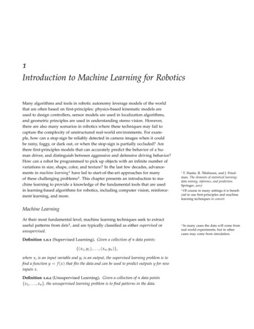
6introduction to machine learning for roboticsvery powerful function approximators. Mathematically, neural networks aretypically described as a sequence of functions:h1 f 1 (W1 x b1 ),h2 f 2 (W2 h1 b2 ),(1.5).ŷ f K (WK hK 1 bK ),which is an easier notation than writing the equivalent composite function:ŷ f K (WK f K 1 (. . . ) bK ).In this model, the parameters are the weights W1 , . . . , WK and biases b1 , . . . , bK ,and the structure of the model is predefined by the choice of the activationfunctions f 1 , . . . , f K and the number of layers K. The intermediate variablesh1 , . . . , hK 1 are the outputs of the hidden layers, aptly named since they arenot the input or the output of the model.To fully specify the structure of the model, a practitioner needs to specify thenumber of hidden layers18 , the dimensionality of each of the intermediate variables hi (usually chosen to be the same for all hidden layers), and the activationfunctions f i .Neural networks with many layersare referred to as deep neural networks.181.3.1 Activation FunctionsCommonly used activation functions f 1 , . . . , f K in neural networks include sigmoid functions, hyperbolic tangent functions, rectified linear units (ReLU), andleaky ReLU functions19 .It is typical for the same activationfunction to be used for all layers of thenetwork.191. Sigmoid function (also denoted as σ ( x )):f (x) 1,(1 e x )2. Hyperbolic tangent function:f ( x ) tanh( x ),3. ReLU function:f ( x ) max{0, x },4. Leaky ReLU function:f ( x ) max{0.1x, x },It is important to note that each of these activation functions share two important characteristics: they are nonlinear and they are easy to differentiate. Itis critical that the activation function be nonlinear since a composition of linear functions will remain linear, and therefore no additional benefit is gainedin modeling capability by adding more than a single layer to the network. Differentiability is also critical because the gradients must be easily computableduring training20 .While ReLU and leaky ReLU are notstrictly differentiable, this issue is easilymitigated in practice.20
principles of robot autonomy1.3.2 Training Neural NetworksNeural networks are trained with gradient-based numerical optimization techniques, such as those mentioned in Section 1.2.1 (e.g. stochastic gradient descent). Therefore once a particular loss function L has been chosen, the gradients L θ must be computed for each parameter. Since neural networks cancontain a large number of parameters, this gradient computation must be accomplished in a computationally efficient way. In particular, the gradients arecomputed using an algorithm referred to as backpropagation, which leverages thechain rule of differentiation and the layered structure of the network.As with other parametric models, it is very important to avoid overfittingwhen training neural networks21 . This can partially be accomplished using thedivision of the dataset into training and test sets, as well as by using regularization techniques as mentioned in Section 1.2.2. Another technique for avoidingoverfitting in neural networks is referred to as dropout, where some “connections” in the network are occasionally removed during the training process. Thisessentially forces the network to learn more redundant representations, whichhas been shown to improve generalization. Of course another useful techniqueto avoid overfitting is just to have an extremely large dataset, but in many casesthis may not be very practical.1.4Figure 1.1: Common activation functions used in neuralnetworks.It is quite easy to overfit when training neural networks since they havesuch a large number of parameters.21Backpropagation and Computational GraphsFrom a theoretical standpoint, computing the gradients dLdθ of the loss functionwith respect to the parameters is relatively straightforward. However, from apractical standpoint computing these gradients can be computationally expensive, especially for complex models such as neural networks. Backpropagation22is an algorithm that addresses this issue by computing all required gradients inan efficient way.Backpropagation computes gradients by cleverly choosing the order in whichoperations required to compute the gradient are performed. By doing so it seeksto avoid redundant computations, and can in fact be viewed as an exampleof dynamic programming. While in some simple cases the backpropagationSometimes also referred to as autodifferentiation.22Many software tools, such as PyTorch(https://pytorch.org/) and TensorFlow (https://www.tensorflow.org/)will automatically be able to performbackpropagation for a large class offunctions.7
8introduction to machine learning for roboticsalgorithm may provide only a small advantage, in many cases (and in particularfor neural network training) backprop can be orders of magnitude faster thannaive approaches.A computational graph is another practical tool that is useful when using thebackpropagation algorithm to compute gradients. A computational graph provides a way to express a mathematical function using representations fromgraph theory. In particular the function is expressed as a directed graph wherethe nodes represent mathematical operations or function inputs and the edgesrepresent intermediate quantities. Using a computational graph, a forward passthrough the graph (starting at the root nodes, which are function inputs) isequivalent to evaluating the function.This representation makes it very easy to see the structure of the mathematical operation that can be exploited by the backpropagation algorithm. As anexample, consider the function L( x, y) g( f ( x, y)) and its associated computational graph shown in Figure 1.2 (which includes the intermediate variabledL zz). Using the chain rule, the gradient of L with respect to x is L x dz x . Thebackpropagation algorithm uses this structure to convert the computation ofdL zthe gradient L x into a sequence of local gradient computations dz and x , corresponding to each computation node in the graph. With this structure redundantcomputation can be be avoided. For example, when computing L y the partialgradientdLdzcan be reused.Figure 1.2: Example computational graph for a functionL( x, y) g( f ( x, y)).To summarize, the backpropagation algorithm follows the following basicsteps:1. Perform a forward pass through the computational graph to compute anyintermediate variables that may be needed for computing local gradients23 .2. Starting from the graph output, perform a backwards pass over the graphwhere at each computation node the local gradient of the node with respectto its inputs and outputs is computed. Then, compute the gradient of thegraph’s output with respect to the inputs of the local computation node,leveraging the chain rule and previously calculated gradients. In Figure 1.2,dgthe first step of backprop would be to compute L z dz , and the second step L Lwould use L z to compute the remaining gradients x and y .Example 1.4.1 (Training a Simple Model). Consider a supervised learning problem with a parametric model defined as:f ( x ) ( x a)( x b),For example if g(z) z2 the gradient 2z depends on the current valueof z23dgdz
principles of robot autonomy9where a and b are parameters of the model, and a l2 loss function (1.1) is usedfor training. A computational graph for computing the loss from a single datapoint with this model is shown in Figure 1.3.For this model and loss function the gradients required for training can becomputed analytically as: Li 2(y ( x a)( x b))( x b), a Li 2(y ( x a)( x b))( x a). bComputing the gradients in this way (the naive approach) would require 7operations each (4 sums and 3 multiplications), for a total of 14 operations.Alternatively the gradients can be computed in a more efficient way usingbackpropagation, which avoids redundant computations. This approach can beviewed as taking a backward pass over the computation graph. Starting at theoutput of the graph: Li 2z1 . z1Then moving on through the next operations and using the chain rule (andreusing the previous computations): Li L z L i 1 i, ŷ z1 ŷ z1and: Li L i z2 ŷ Li L i z3 ŷ ŷ L i z3 , z2 ŷ ŷ L i z2 . z3 ŷFinally, the next step backward reaches the parameters a and b: Li L z L i 2 i, a z2 a z2 Li L z L i 3 i. b z3 b z3To actually compute the numerical values of these gradients:1. First perform a forward pass through the network to compute the values z1 ,z2 , and z3 (5 operations).2. Then perform the backward pass computations to compute Li a ,and Li b Li Li Li Li z1 , ŷ , z2 , z3 ,(4 operations).Using backpropagation, only 9 operations are required to compute the gradients Li Li a , and b , which is a non-negligible reduction over the naive approach!Figure 1.3: Computationalgraph for computing the lossfor a single data point for themodel f ( x ) ( x a)( x b)with l2 loss (see Example 1.4.1).The values ( xi , yi ) are the datapoint, the model output is ŷ,and z1 , z2 , z3 are intermediatevariables. The quantities a andb are parameters of the model.
4 introduction to machine learning for robotics Example 1.2.1 (Linear Least Squares). One of the most fundamental regression problems, linear least squares, can be solved analytically. In this problem, the parametric model is a linear model11: 11 This approach can also be extended