Transcription
Analysis of Manufacturing Systemsusing Chi 3.0I.J.B.F. Adan, A.T. Hofkamp, J.E. Rooda and J. VervoortOct 2012Technische Universiteit Eindhoven, Department of Mechanical EngineeringSystems Engineering Group, P.O. Box 513, 5600 MB Eindhoven, The Netherlandshttp://se.wtb.tue.nl/a.t.hofkamp@tue.nl
ii
ContentsAcknowledgementsvii1 Introduction11.1Manufacturing Systems (MSs) . . . . . . . . . . . . . . . . . . . . . . . . . . .11.2Analysis of Manufacturing Systems (AMS)3. . . . . . . . . . . . . . . . . . .2 Analytical models of deterministic manufacturing systems72.1Manufacturing system principles . . . . . . . . . . . . . . . . . . . . . . . . .72.2Analysis of deterministic manufacturing systems . . . . . . . . . . . . . . . . 132.3Exercises2.4Additional exercises . . . . . . . . . . . . . . . . . . . . . . . . . . . . . . . . 27. . . . . . . . . . . . . . . . . . . . . . . . . . . . . . . . . . . . . . 243 Analytical models of stochastic manufacturing systems313.1Classification of manufacturing queueing models . . . . . . . . . . . . . . . . 313.2Queueing relations for single-machine workstation . . . . . . . . . . . . . . . . 323.3Queueing relations for a flowline . . . . . . . . . . . . . . . . . . . . . . . . . 353.4Identical parallel machines . . . . . . . . . . . . . . . . . . . . . . . . . . . . . 373.5Batch machines . . . . . . . . . . . . . . . . . . . . . . . . . . . . . . . . . . . 393.6Discussion . . . . . . . . . . . . . . . . . . . . . . . . . . . . . . . . . . . . . . 413.7Exercises. . . . . . . . . . . . . . . . . . . . . . . . . . . . . . . . . . . . . . 434 Single workstation474.1Single machine model . . . . . . . . . . . . . . . . . . . . . . . . . . . . . . . 474.2Single machine with varying process time . . . . . . . . . . . . . . . . . . . . 494.3Single machine with buffer4.4Displaying simulated behaviour . . . . . . . . . . . . . . . . . . . . . . . . . . 544.5Exercises. . . . . . . . . . . . . . . . . . . . . . . . . . . . 51. . . . . . . . . . . . . . . . . . . . . . . . . . . . . . . . . . . . . . 56iii
ivContents5 Measuring performance615.1Mean throughput . . . . . . . . . . . . . . . . . . . . . . . . . . . . . . . . . . 615.2Mean flowtime . . . . . . . . . . . . . . . . . . . . . . . . . . . . . . . . . . . 625.3Mean utilization . . . . . . . . . . . . . . . . . . . . . . . . . . . . . . . . . . 645.4Mean wip-level . . . . . . . . . . . . . . . . . . . . . . . . . . . . . . . . . . . 665.5Variance . . . . . . . . . . . . . . . . . . . . . . . . . . . . . . . . . . . . . . . 685.6Measuring other quantities5.7Simulation vs Approximation (1): single machine workstation . . . . . . . . . 695.8Discussion . . . . . . . . . . . . . . . . . . . . . . . . . . . . . . . . . . . . . . 715.9Exercises. . . . . . . . . . . . . . . . . . . . . . . . . . . . 69. . . . . . . . . . . . . . . . . . . . . . . . . . . . . . . . . . . . . . 716 Machines in series736.1Deterministic flowline . . . . . . . . . . . . . . . . . . . . . . . . . . . . . . . 736.2Unbalanced flowline . . . . . . . . . . . . . . . . . . . . . . . . . . . . . . . . 776.3Machines in series without buffers6.4Simulation vs Approximation (2): flowline . . . . . . . . . . . . . . . . . . . . 796.5Exercises6.6Case . . . . . . . . . . . . . . . . . . . . . . . . . . . . . . . . . . . . . . . . . 88. . . . . . . . . . . . . . . . . . . . . . . . 78. . . . . . . . . . . . . . . . . . . . . . . . . . . . . . . . . . . . . . 837 Machines in parallel917.1Deterministic machines in parallel . . . . . . . . . . . . . . . . . . . . . . . . 917.2Analytical vs Simulation (3): Parallel machines . . . . . . . . . . . . . . . . . 937.3Parallel machines for different lot types . . . . . . . . . . . . . . . . . . . . . 947.4Exercises. . . . . . . . . . . . . . . . . . . . . . . . . . . . . . . . . . . . . . 978 Other configurations998.1Bypassing . . . . . . . . . . . . . . . . . . . . . . . . . . . . . . . . . . . . . . 1008.2Backtracking . . . . . . . . . . . . . . . . . . . . . . . . . . . . . . . . . . . . 1038.3Assembly line . . . . . . . . . . . . . . . . . . . . . . . . . . . . . . . . . . . . 1068.4Jobshop . . . . . . . . . . . . . . . . . . . . . . . . . . . . . . . . . . . . . . . 1088.5Exercises. . . . . . . . . . . . . . . . . . . . . . . . . . . . . . . . . . . . . . 1119 Extending machine models1179.1Representing process time by a distribution . . . . . . . . . . . . . . . . . . . 1179.2Machine failure and repair . . . . . . . . . . . . . . . . . . . . . . . . . . . . . 127
Contents10 Case: (Part of ) a waferfabv13510.1 The manufacturing of Integrated Circuits (ICs) . . . . . . . . . . . . . . . . . 13610.2 Wafer processing . . . . . . . . . . . . . . . . . . . . . . . . . . . . . . . . . . 13610.3 The oxide furnace and lithographic equipment . . . . . . . . . . . . . . . . . . 13810.4 Analytical approach . . . . . . . . . . . . . . . . . . . . . . . . . . . . . . . . 13910.5 Simulation-based analysis . . . . . . . . . . . . . . . . . . . . . . . . . . . . . 141Bibliography145
viContents
AcknowledgementsThis book is the result of years of research within the Systems Engineering Group of theDepartment of Mechanical Engineering of the Eindhoven University of Technology. Creditsfor the design of the language go to all members of the χ-club. In particular, we would liketo mention the following contributions. J.M. van de Mortel-Fronczak stood at the base ofthe language [vdMFR95]. N.W.A. Arends was the first to describe the formalism [Are96].W. Alberts and G.A. Naumoski wrote the first compiler (χ0.3) [AN98]. A.T. Hofkamp wrotethe real-time compiling system [Hof01] and the latest compiler (Chi 3). V. Bos and J.J.T.Kleijn helped in providing a formal framework for χ [BK00]. D.A. van Beek gave suggestionsfor improving the language. Finally, close cooperation of the Systems Engineering Groupwith the Parallel Programming Group (formerly lead by M. Rem) and the Formal MethodsGroup (lead by J.C. Baeten) has improved the quality of the language.In addition, we would like to thank all (former) students and (former) members of theSystems Engineering Group that have performed several projects involving the modellingand analysis of manufacturing systems using Chi in research and engineering environments.Regarding this book, we thank L.F.P. Etman for his contribution to Chapter 3 and forpreparing a number of exercises. We thank E.J.J. van Campen for providing us with photographs of the Crolles2 waferfab.Chi 3This edition is based on the language Chi 3. The original text has been modified, withminimal effort, to make the text suitable for Chi 3.Some chapters have been deleted from this edition.vii
viiiAcknowledgements
Chapter 1IntroductionThe title of this book is analysis of manufacturing systems. In this chapter we mark outthe main focus of the book.1.1Manufacturing Systems (MSs)Manufacturing stems from the Latin words manus (hand) and factus (make). Nowadays,by manufacturing we mean the process of converting raw material into a physical product(we do not consider services to be manufacturable). A system is a collection of elementsforming a unified whole. Thus, a manufacturing system refers to any collection of elementsthat converts raw material into a product. We can identify manufacturing systems at fourdifferent levels. At factory level the manufacturing system is the factory (also referred to as plant,fabricator, or shortly fab). The elements of the system are areas and (groups of)machines. At area level the manufacturing system is an area of the factory with several machinesor groups of machines (cells). The elements of the system are individual machines. At cell level the manufacturing system is a group of machines, that are typicallyscheduled as one entity. At machine level, the manufacturing system is the individual machine (also referredto as equipment or tools). The elements of the system are machine components.These levels constitute a hierarchical breakdown of the factory, see Figure 1.1.In this book we will focus on manufacturing systems at area and cell level. Though, manyparts of this book are also applicable to analysis of entire factories or individual machines.For instance, the analysis of the output (for instance the number of products processed perhour) of a factory shows many similarities to analyzing the output of an area, or the outputof machine. Scheduling tasks at machine level is in many ways analogous to schedulingorders at factory level or scheduling jobs at area level.1
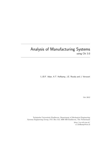
2Chapter 1. IntroductionLevel4 factory3 area2manufacturingcell1 machineFigure 1.1: Manufacturing systems regarded at different levelsThe types of manufacturing systems that can be analyzed using the approach described inthis book are as diverse as there are products. Some examples are: a wafer fab (factory level), the lithography area (area level), a waferstepper (machine),see Figures 1.2 and 1.3, a CD-R fab (factory level), the CD-R mastering area (area level), a CD-R printingmachine(machine level), see Figure 1.4, an automotive assembly factory (factory level), the bodywork assembly line (arealevel), the welding robots (cell level), a single welding robot (machine level), see Figure 1.5.Figure 1.2: Lithographic area of the Crolles2 waferfab in Grenoble, FranceFigure 1.3: Waferinspection machine and waferstepper in the lithographic area of theCrolles2 waferfab
1.2. Analysis of Manufacturing Systems (AMS)3Figure 1.4: CD optical mastering area, CD printing machine, CD packaging machine (source:http://www.sonopress.de)Figure 1.5: Automotive assembly line (source: http://www.mazda.com)In this book we consider different types of manufacturing systems. Depending on the specificindustry we are in, we see for example shoes, a pod of wafers, or a printed-circuit boardmoving through the factory. Throughout this book we use the term lot to refer to thecommon transfer unit in the manufacturing system. If a machine processes multiple lots atthe same time, we say the machine processes batches. A batch is a set of lots.1.2Analysis of Manufacturing Systems (AMS)Some typical design questions when designing or optimizing a manufacturing system are: What machines do I choose? Do I choose a cheap machine that breaks down often, ora more expensive machine, that breaks down less often? How many machines do I use? Do I choose a single high-capacity machine, do I choosemultiple low-capacity machines in parallel, or a combination? What configuration of workstations do I choose? Do I choose a flowline, a jobshop, orsomething in between? Do I want buffers and if so of what size? What control strategy do I use for my plant? Do I release new orders at a fixed rateand if so at what rate? Do I release orders according to a precalculated schedule ordo I release orders based on the plant status?
4Chapter 1. IntroductionThis book does not go into much detail on the best answers, but presents a way to model andanalyze a manufacturing system to help you answer these questions yourself. We analyzemanufacturing systems with one objective: to evaluate and compare alternative manufacturing system designs and decide on the best alternative.Question is: on what criteria do we evaluate and compare manufacturing systems? Manydifferent performance criteria exist. Some commonly used performance indicators are: throughput δ: the number of lots per time-unit that leave the manufacturing system, flowtime ϕ: the time it takes a lot to travel through the system, coefficient of variation on the flowtime (cϕ ): the amount of variability on the flowtimeof a lot, utilisation u: the fraction of time a machine is processing lots, and work-in-process or wip-level w: the number of lots in the manufacturing system.More on these and other performance indicators can be found in [GH85], [Tij94], [HS01]and in the remainder of this book.In order to analyze a (design of a) manufacturing system, we need a way to model it and todetermine its performance. We can make many different types of models. Often it is possibleto make a rough estimation of the plant performance without requiring advanced modelling,see for example [HS01]. In the early stages of the design process we often can not do betterthan rough estimates, since we do not have enough detailed data. As we collect more data,it is possible, for simple plants, to do some more accurate calculations with simple queueingequations, see again [GH85, Tij94]. However, these queueing equations have a limited rangeof application and validity. If plants become more complex, we require advanced queuingtheory (as can be found in for example [GH85, BS93, Tij94, AR01]) and stochastic processtheory. However, these models require extensive mathematical knowledge, substantial effort,and even these models have a limited range of applicability. Here, we can no longer useanalytical models1 and we enter the field of (discrete-event) simulation. Figure 1.6 showsthe stage in the design process, the amount of data needed, and the range of applicabilityrelated to the analysis methods mentioned.Many commercial simulation packages are available that use computer power to calculateand predict the performance of the plant. These packages offer ready-to-use parametricbuilding blocks of plant components such as machines and buffers. Examples are Flexsim[Fle02], Witness [Lan02], Automod [Bro03], Simscript II.5 [Cac02], and Extend 5.0 [Ima02].However, when plants become more complex and components become more unconventional(due to for example batching policies, control strategies, specific routings, uncommonly useddistributions), substantial low-level programming (in for example C or C ) is requiredand modelling and simulation become time consuming. Then, also these packages reach theboundaries of their applicability.In this book, we propose a way to analyze manufacturing systems using the formalismChi. The Chi-language can be used for modelling and simulating simple manufacturingsystems, but is especially valuable for modelling and simulating complex manufacturingsystems. It offers a high degree of freedom, without requiring extensive programming effort.1 By analytical models we mean mathematical models that can (sometimes only after a significant amountof effort) be explicitly solved and yield an exact solution.
1.2. Analysis of Manufacturing Systems (AMS)design stageearly5Rough estimateSimple Queueing EquationsQueueing Equations withextensions for:- batching- series and setup-time- failureAdvanced queuing theory andstochastic process theoryDiscrete-event simulationfinalamount ofdata neededrange ofapplicabilityFigure 1.6: Different analysis methodsChi is a high-level formalism, tailored to describe concurrent behaviour (which typicallyis the case in plants). The Chi-language is based on computer science and mathematics[BW90, Fok00, Bru97]. It has been used in numerous cases to analyze the performanceand behaviour of complex manufacturing systems. Examples are semi-conductor factories,chemical plants, automobile assembly lines, and factories for lithographic equipment as wellas lithographic equipment itself, wafer furnaces, or a chemical clinical analyzer.On reading this bookReaders familiar with the Chi-language can simply start at Chapter 2 and go from there.Readers unfamiliar with the Chi-language can familiarize themselves with it, by workingthrough the ”Chi 3 tutorial” [AHR12]. In the beginning of each chapter in this book, weindicate what elements of the Chi-language are required to understand the models that arepresented.Each chapter contains a number of exercises. Answers to some of these exercises are includedin the back of this book.OutlineThe structure of this book is as follows. In Chapter 2 we discuss easy-to-use analyticalways to analyze a deterministic manufacturing system. In Chapter 3 we discuss analyticalapproaches to analyze stochastic manufacturing systems, for example with stochastic processtimes.In Chapter 4 we start with modelling a single machine flowline. We present a basic modelof a buffer and a machine. Then, in Chapter 5, we present a way to measure performance ofa manufacturing system by simulation, amongst others, how to measure mean throughput,flowtime and utilisation. In Chapter 6, we continue with analyzing flowlines of multiplemachines with and without buffering. Subsequently, in Chapters 7 and Chapter 8, we discuss the modelling and analysis of networks of machines, for example, parallel machines,jobshops, and re-entrant flowlines. Subsequently, in Chapter 9, we present ways to extendand improve machine models. We discuss aspects like more advanced distributions to represent the process time, adding machine failure and repair, and modelling batching and
6Chapter 1. Introductionset-up times. In the final chapters we present a number of industrial cases, in which theChi-language was used to analyze manufacturing systems.
Chapter 2Analytical models ofdeterministic manufacturingsystemsIn Chapter 1 we saw that there are different ways to analyze a manufacturing system. Inthis chapter and the following chapter, we provide a brief view on analytical models thatcan be used to analyze manufacturing systems. We distinguish two classes of analyticalmodels: deterministic and stochastic models.A variable is deterministic if we know in advance what exact value it has and will have atevery instant of time, that is, the value of the variable is predetermined. A constant deterministic variable is simply a constant, e.g. 1.54. A dynamic deterministic variable changes,but the changes are known in advance, for example a fixed sequence: {1,5,1,5,1,5,1,5}. Avariable is stochastic if we do not know the exact value of the variable in advance. We onlyknow its value obeys some probability distribution. An example of stochastic variable is asample of a binomial distribution: {1,0,1,0,1,1,1,0,0,1}.In this chapter we discuss the principles of manufacturing system analysis and presentanalytical approaches to analyze deterministic manufacturing systems. In Chapter 3 wepresent analytical approaches to analyze stochastic manufacturing systems.In the subsequent chapters we occasionally compare the results of the analytical methodsdiscussed in this and the subsequent chapter with simulation results to investigate the (rangeof) validity of the analytical approaches in an engineering environment.2.1Manufacturing system principlesBefore we introduce analytical models of manufacturing systems, we first introduce a fewbasic quantities and the main principles for manufacturing system analysis.7
8Chapter 2. Analytical models of deterministic manufacturing systemsBasic quantitiesIn this section we present the following basic quantities: raw process time t0 , throughput δ,flowtime ϕ, wip (work-in-process) w, and utilisation u. Other quantities exist, but are dealtwith when encountered in the remainder of the book. Figure 2.1 illustrates throughput,flowtime, wip, and utilisation for manufacturing systems at factory and machine level.j [hours]d [lots/hour]factorylevelw [lots]j [hours]d [lots/hour]buffermachinelevelt0 [hours]w [lots]Figure 2.1: Basic quantities for manufacturing systems Raw process time t0 denotes the net time a lot needs processing on a machine. Thisprocess time excludes additions such as setup time, breakdown, or other sources thatmay increase the time a lot is on the machine. The raw process time is typicallymeasured in hours or minutes. Throughput δ denotes the number of lots per time-unit that leaves the manufacturingsystem. At machine level, this denotes the number of lots that leave a machine pertime-unit. At factory level it denotes the number of lots that leave the factory pertime-unit. The unit of throughput is typically lots/hour. Flowtime ϕ denotes the time a lot is in the manufacturing system. At factory levelthis is the time from release of the lot in the factory until the finished lot leaves thefactory. At machine level this is the time from entering the machine (or the bufferin front of the machine) until leaving the machine. Flowtime is typically measured indays, hours, or minutes. Wip-level w denotes the total number of lots in the manufacturing system, i.e. in thefactory or in the machine. Wip is measured in lots. Utilisation u denotes the fraction a machine is not idle. A machine is considered idle ifit could start processing a new lot. Thus processing time as well as downtime, setuptime and preventive maintenance time all contribute to the utilisation. Utilisation hasno dimension. Utilisation can never exceed 1.0.
2.1. Manufacturing system principles9In literature different formulas are presented to compute the utilisation in specific cases.We present only one formula:u TnonidleTtotal(2.1)Herein Tnonidle denotes the time the machine is not idle during a total timeframe Ttotal . Inthe following examples we calculate the utilisation for a number of cases.Example 2.1 Utilisation (1)A machine has raw process time t0 of 0.15 hours and processes 5 lots/hour. Calculate theutilisation.Processing 5 lots takes 5 0.15 0.75 hours. Every hour the machine is idle for 0.25 hours,hence utilisation u 0.75. Example 2.2 Utilisation (2)A machine has raw process time t0 0.15 hours. Lots arrive at a fixed rate of 5.0 lots/hour.After every fourth lot, the machine needs recalibrating. Recalibration takes 0.10 hour.Calculate the utilisation.To process four lots, the machine is occupied for 4 0.15 0.10 0.70 hours. Theselots are processed over a total time of 4/5.0 0.80 hours. Hence the mean utilisation is0.7/0.8 0.875. Example 2.3 Utilisation for batch processingA machine processes lots in fixed batches1 . Processing a batch takes 3 hours. After everybatch the machine needs to be cleaned and prepared for the next batch, which takes 1 hour.Lots arrive at a rate of 2 lots/hour. Calculate the utilisation for a batch size of 10 and 12lots respectively.2 lots/hourbatchmachineFigure 2.2: Batch machine processing in batches of 10 lotsIn case of a batch size of 10 lots, the machine processes a batch every 5 hours. For everybatch the machine is occupied for 3 1 4 hours. The machine is idle for 1 hour every5 hours, the utilization u 4/5 0.80. In case of a batch size of 12 lots, the machineprocesses a batch every 6 hours. The utilisation is now u 4/6 0.67. First principle: Conservation of massThe first principle for manufacturing systems is conservation of mass. Similar as for fluidflow systems, conservation of mass applies to manufacturing systems. Figure 2.3(a) showsa workstation (buffer and machine). Herein λ1 denotes the arrival rate in lots/hour, δ11Abatch is a set of lots processed together.
10Chapter 2. Analytical models of deterministic manufacturing systemsdenotes the throughput in lots/hour and w1 denotes the number of lots in the workstation. InFigure 2.3(b), the total throughput δ1 of workstation 1 splits into two flows, with throughputrates δ1,1 and δ1,2 respectively. In Figure 2.3(c), λ2,1 and λ2,2 together form the total arrivalrate of workstation 2.w1l1w1d1l1d1,1l2,11d22d1,2(b)(a)w2l2,2(c)Figure 2.3: Three workstationsConservation of mass for Figure 2.3(a) yields:dw1 λ1 δ 1dt(2.2)This differential form of mass conservation states that the change in the number of lotsdw/dt in workstation 1 is equal to the number of lots entering workstation 1 minus thethe number of lots leaving workstation 1 per unit of time. On many occasions we considersystems in steady state. We say a manufacturing system is in steady state when the meannumber of lots in the system is constant, that is, there are no lots piling up in the system,or dw/dt 0. In this case, the mean number of lots entering the manufacturing systemequals the mean number of lots leaving the system. Equation 2.2 becomes:λ1 δ 1 0(2.3)Herein λ1 and δ1 represent the mean arrival rate and throughput in steady state. For theworkstations in Figure 2.3(b) and (c), mass conservation in steady state yields:λ1 δ1,1 δ1,2 0λ2,1 λ2,2 δ2 0(2.4)We denote the total throughput of workstation 1 as δ1 δ1,1 δ1,2 . Moreover, we haveconsidered workstations here, but we can just as well consider factories or areas.Example 2.4 Manufacturing areasFigure 2.4 shows a factory consisting of 6 areas and the raw processing time of every area.Area 1 receives 3 lots/hour. After being processed in Area 1, 40% of all lots are processedin Area 2 and 3, and 60% of all lots are processed in Area 4 and 5. Finally all lots areprocessed in Area 6. Consider the factory in steady state and calculate the throughput ofArea 2 and 4 and the utilisation for all 6 areas.The throughput rates for Areas 2 and 4 follow directly from the given probability data:δ2 0.4 · λ1 0.4 · 3 1.2 lots/hourδ4 0.6 · λ1 0.6 · 3 1.8 lots/hourArea 1 processes 3 lots/hour. Processing 3 lots per hour in Area 1 takes 3 · 0.2 0.6 hours.Every hour, the area is occupied for 0.6 hours, hence utilisation u1 0.6.
2.1. Manufacturing system principles11Area20.4l1 3 lots/hour1d6640.612345635t0 [hrs]0.20.60.40.30.40.3Figure 2.4: Material flow in six manufacturing areasArea 2 processes 1.2 lots/hour. Processing 1.2 lots in Area 2 takes 1.2 · 0.6 0.72 hours,hence utilisation u2 0.72.In a similar way, we calculate the utilisation for the remaining areas. u3 0.48, u4 0.54,u5 0.72, and u6 0.9. As all utilisations are smaller than 1, lots do not pile up in thissystem. Example 2.5 ReworkConsider the manufacturing system in Figure 2.5(a). The manufacturing system consists oftwo infinite buffers (B1 and B2 ) and two machines (M1 and M2 ). 50% of the lots processedby machine 1 need to be reprocessed by machine 1. 25% of the lots processed by machine2, have to be reprocessed by machine 1 and 2 again. Lots arrive at machine 1 with a fixedarrival rate of 3 lots/hour. Calculate (a) the number of lots that machine 1 processes perhour and (b) the number of lots that leave the system via machine 2. Assume that thesystem is in steady state.dM2B125%3 lots/hrB1M150%B2M275%lB1 3 lots/hrB1dB1M1dM1B2B2dB2M2dM2EdM1B150%(a)(b)Figure 2.5: Manufacturing line with reworkThe total throughput of machine 1 splits into two flows. We introduce throughput δM1 B1and δM1 B2 , denoting the number of lots/hour that are sent from machine M1 back to thefirst buffer B1 and from machine M1 forward to the second buffer B2 respectively. Weintroduce additional throughput rates, see Figure 2.5(b). Throughput δM2 E denotes thenumber of lots per hour that exit the system after being processed by machine M2 . Frommass conservation and the probability data, we obtain the following equations:B1M1B2M2λ B1 δ M 1 B1 δ M 2 B1 δ B1 0δM1 B2 δM1 B1 0.5δB1δ B2 δ M 1 B2δM2 E 0.75δB2δM2 B1 0.25δB2Filling in (2), (3), and (4) in (1) leads to:λB1 0.5δB1 0.25δB2 δB1 0λB1 0.5δB1 0.25δM1 B2 δB1 0(1)(2)(3)(4a)(4b)
12Chapter 2. Analytical models of deterministic manufacturing systemsλB1 0.5δB1 0.125δB1 δB1 0δB1 83 λB1 8 lots/hourThus 8 lots/hour enter machine M1 . In steady state, M1 processes 8 lots/hour. Of these 8lots/hour, 4 lots/hour proceed to buffer B2 and 4 lots/hour are lead back to buffer B1 .The number of finished lots that leave the system after being processed on machine M2 is:δ M2 E 0.75δB2 0.75δM1 B2 83 δB1 3 lots/hourThe throughput of this line is 3 lots/hour. Note that the number of lots entering the line isequal to the number of lots leaving the line. Due to rework, machine M1 has to process 8lots/hour. Second principle: Little’s lawThe second principle for manufacturing systems is Little’s law. Little’s law states that themean wip-level (number of lots in a manufacturing system) w is equal to the product of themean throughput δ and the mean flowtime ϕ [Lit61], provided the system is in steady state.w δ·ϕ(2.5)This can be intuitively interpreted by looking at Figure 2.6, which treats a manufacturingsystem as a pipeline where lots pass through. The total amount of fluid in the pipeline in[m3 ] is equal to the flowrate in [m3 /s] multiplied by the time it takes an imaginary fluidelement to flow through the pipe in [s].dwjFigure 2.6: Manufacturing system as pipelineAnalogously, the mean number of lots in a manufacturing system (wip-level w in [lots]) isequal to the mean number of lots leaving the system per unit of time (throughput δ in[lots/timeunit]) multiplied by the mean time a lot remains in the system (flowtime ϕ in[timeunits]). Little’s law only applies in steady state.Example 2.6 Automotive factoryWe study the automotive factory in Figure 2.7. By simple measurements we determine that
2.2. Analysis of deterministic manufacturing systems1325 days200 cars/dayFigure 2.7: Automotive factory200 cars per day leave the factory. On average a car (or its parts) stay for 25 days in thefactory. Calculate the mean number of cars in the factory in steady state.By Little’s law we estimate that the factory contains w δ · ϕ 200 · 25 5000 cars (orparts for 5000 cars). Example 2.7 AreasA factory has four areas. 50% of the lots are processed in Area 1, 2, and 3. The remaining50% is processed in Area 1 and 4. Through the year, we count the number of (semi-finished)lots in each area. The mean number of lots in each area are shown in Figure 2.8. Moreover,new lots arrive at Area 1 with a an arrival rate λ 10 lots/hour. Calculate the meanflowtime per area.10 lots/hour15 lots/hour25 lots/hour34Area1234w100120100240Figure 2.8: Factory with four areasWith Little’s law we calculate the mean flowtime per area.ϕ1 w1 /δ1 100/10 10 hoursϕ2 w2 /δ2 120/5 24 hoursϕ3 w3 /δ3 100/5 20 hoursϕ4 w4 /δ4 240/5 48 hours 2.2Analysis of deterministic manufacturing systemsIn this section we explore the possibility to estimate the performance of a factory (or area),without detailed data and/or extensive calculations. We analyze problems where:1. the machi
The title of this book is analysis of manufacturing systems. In this chapter we mark out the main focus of the book. 1.1 Manufacturing Systems (MSs) Manufacturing stems from the Latin words manus (hand) and factus (make). Nowadays, by manufacturing we mean the p