Transcription
How to Handle Binomial Proportion with Zero FrequencyTulin Shekar, Merck & Co., Inc., Whitehouse Station, NJABSTRACTEstimating confidence interval for the binomial proportion is a challenge to statisticians and programmers whenthe proportion has zero frequency. This paper reviews the statistical methods used for estimating confidence intervals which are available in SAS . The observations with zero frequency treated as missing by SAS and notpresented in the output.Application of the macro developed to clinical trial Adverse Event data, specifically on how to create confidenceintervals with zero frequency will be provided.KEY WORDSBinomial Proportion, Confidence Intervals, Zero Frequency, SAS Macro.INTRODUCTIONIn clinical trials, the incidence rates of pre-specified Adverse Events are often of interest due to safety concerns.Some examples might include BP(Blood Pressure) and transaminase (AST or ALT) parameters such as the proportion of subjects who have any incidence of systolic BP 180 mm Hg, diastolic BP 105 mm Hg, AST 3 x ULNwith 10% increase from Baseline or ALT 3 x ULN with 10% increase from Baseline. Presentation of 95% CI’sfor the incidence rates for AE events of interest using exact approach will be the primary interest for this paper.A binary response is a typical example, which has 0 (non-response) and 1 (response). Define X as the frequencyof the first (or designated) level and n as the total frequency of the one-way table. The binomial proportion for agiven endpoint and treatment is computed asp̂ X / nDenote by zα / 2 the 100(1 α / 2) th percentile of the standard normal distribution.Several methods to estimate the confidence interval for the binomial proportion (we focus on two-sided intervals here) are as follows: Wald asymptotic confidence interval:The simplest and most commonly used formula for a binomial confidence interval relies on approximating the binomial distribution with a normal distribution. This approximation is justified by the central limit theorem. The formula iswheretheis the proportion of successes in a Bernoulli trial process estimated from the statistical sample,percentile of a standard normal distribution,isis the error percentile and n is the sample size.The central limit theorem applies well to a binomial distribution, even with a sample size less than 30, aslong as the proportion is not too close to 0 or 1. For very extreme probabilities, though, a sample size of 30 ormore may still be inadequate. The normal approximation fails totally when the sample proportion is exactly zero or1
exactly one. A frequently cited rule of thumb is that the normal approximation works well as long as np 5 andn(1 p) 5; see however Brown et al. 2001. In practice there is little reason to use this method rather than one ofthe other, better performing, methods.An important theoretical derivation of this confidence interval involves the inversion of a hypothesis test. Underthis formulation, the confidence interval represents those values of the population parameter that would havelarge p-values if they were tested as a hypothesized population proportion. The collection of values,𝜃 for whichthe normal approximation is valid can be represented asSince the test in the middle of the inequality is a Wald test, the normal approximation interval is sometimes calledthe Wald interval. Agresti-Coull confidence interval:The Agresti-Coull interval is another approximate binomial confidence interval.Givensuccesses intrials, defineandThen, a confidence interval forwhere is theis given bypercentile of a standard normal distribution, as before.Jeffreys confidence interval:The Jeffreys interval is the Bayesian credible interval obtained when using the non-informative Jeffreys prior forthe binomial proportion p. The Jeffreys prior for this problem is a Beta distribution with parameters (1/2, 1/2). Afterobserving x successes in n trials, the posterior distribution for p is a Beta distribution with parameters (X 1/2, n –X 1/2).When x 0 and x n, the Jeffreys interval is taken to be the 100(1 – α)% equal-tailed posterior probability interval,i.e., the α / 2 and 1 – α / 2 quantiles of a Beta distribution with parameters (X 1/2, n – X 1/2). These quantilesneed to be computed numerically, although this is reasonably simple with modern statistical software.2
In order to avoid the coverage probability tending to zero when p 0 or 1, when X 0 the upper limit is calculated as before but the lower limit is set to 0, and when X n the lower limit is calculated as before but the upperlimit is set to 1. Exact (Clopper-Pearson) confidence interval:The Clopper-Pearson interval is an early and very common method for calculating binomial confidence intervals.This is often called an 'exact' method, but that is because it is based on the cumulative probabilities of thebinomial distribution (i.e., exactly the correct distribution rather than an approximation), but the intervals are notexact in the way that one might assume: the discontinuous nature of the binomial distribution precludes any interval with exact coverage for all population proportions. The Clopper-Pearson interval can be written aswhere X is the number of successes observed in the sample and Bin(n; θ) is a binomial random variable with ntrials and probability of success θ.Because of a relationship between the cumulative binomial distribution and the beta distribution, the ClopperPearson interval is sometimes presented in an alternate format that uses quantiles from the beta distribution.where x is the number of successes, n is the number of trials, and B(p; v,w) is the pth quantile from a beta distribution with shape parameters v and w. The beta distribution is, in turn, related to the F-distribution so a third formulation of the Clopper-Pearson interval can be written using F percentiles:where x is the number of successes, n is the number of trials, and F(c; d1, d2) is the 1 - c quantile from an Fdistribution with d1 and d2 degrees of freedom.The Clopper-Pearson interval is an exact interval since it is based directly on the binomial distribution rather thanany approximation to the binomial distribution. This interval never has less than the nominal coverage for anypopulation proportion, but that means that it is usually conservative. For example, the true coverage rate of a 95%Clopper-Pearson interval may be well above 95%, depending on n and θ. Thus the interval may be wider than itneeds to be to achieve 95% confidence. In contrast, it is worth noting that other confidence bounds may be narrower than their nominal confidence with, i.e., the Normal Approximation (or "Standard") Interval, Wilson Interval,Agresti-Coull Interval, etc., with a nominal coverage of 95% may in fact cover less than 95% Wilson (score) confidence interval:The Wilson interval is an improvement (the actual coverage probability is closer to the nominal value) over thenormal approximation interval and was first developed by Edwin Bidwell Wilson (1927).3
This interval has good properties even for a small number of trials and/or an extreme probability. The center of theWilson intervalcan be shown to be a weighted average ofand , with receiving greater weight as the sample sizeincreases. For the 95% interval, the Wilson interval is nearly identical to the normal approximation interval usinginstead of.The Wilson interval can be derived from Pearson's chi-squared test with two categories. The resulting intervalcan then be solved for to produce the Wilson interval. The test in the middle of the inequality is a score test, sothe Wilson interval is sometimes called the Wilson score interval.The Jeffreys interval has a Bayesian derivation, but it has good frequentist properties. In particular, it has coverage properties that are similar to the Wilson interval, but it is one of the few intervals with the advantage of beingequal-tailed (e.g., for a 95% confidence interval, the probabilities of the interval lying above or below the true value are both close to 2.5%). In contrast, the Wilson interval has a systematic bias such that it is centered too closeto p 0.5.For zero frequency observed, that is X 0 (no event), the simplest and most widely used Wald asymptotic gives adegenerate interval, that is, (0, 0), which has the poorest coverage probability among all of these methods. Notethe Wald asymptotic method and all other four methods are recommended for calculating confidence intervals forthe binomial proportions. In the case of binomial proportion with zero frequency, Agresti-Coull always gives thelongest confidence interval, while Jeffreys gives the shortest.Wilson (score) and Clopper-Pearson confidence intervals are widely used in clinical trial analysis. For large sample sizes they both equally perform well. For this paper Clopper-Pearson confidence interval will be used in thegeneration of examples.Prior to SAS 9.1.3, PROC FREQ procedure only provided the Wald asymptotic and exact (Clopper-Pearson)confidence intervals for the binomial proportion. In SAS 9.3, when one specify the BINOMIAL (ALL) option in theTABLES statement, then all of five confidence intervals mentioned in this paper will be provided by SAS. Further,one can specify AC (Agresti-Coull), EXACT(Clopper-Pearson), J (Jeffreys), W (Wilson score) and WALD (Waldasymptotic) in order to obtain the CI’s for these specific methods. Below is the summary of options available inSAS 9.3.4
BINOMIAL (binomial-options) requests the binomial proportion for one-way tables. When you specify the BINOMIAL option, by defaultPROC FREQ also provides the asymptotic standard error, asymptotic (Wald) and exact (ClopperPearson) confidence limits, and the asymptotic equality test for the binomial proportion.Table BINOMIAL OptionsOptionDescriptionRequest Confidence LimitsAGRESTICOULL ACRequests Agresti-Coull confidence limitsALLRequests all confidence limitsEXACT CLOPPERPEARSON Requests Clopper-Pearson confidence limitsJEFFREYS JRequests Jeffreys confidence limitsWALDRequests Wald confidence limitsWILSON WRequests Wilson (score) confidence limitsYou can specify the following binomial-options inside parentheses following the BINOMIAL option:AGRESTICOULL AC: requests Agresti-Coull confidence limits for the binomial proportion.ALL: requests all available types of confidence limits for the binomial proportion. These include the following: Agresti-Coull, exact (Clopper-Pearson), Jeffreys, Wald, and Wilson (score) confidence limits.EXACT CLOPPERPEARSON: requests exact (Clopper-Pearson) confidence limits for the binomial proportion. If you do not request any binomial confidence limits by specifying binomial-options, PROC FREQproduces Wald and exact (Clopper-Pearson) confidence limits by default. To request exact tests for thebinomial proportion, specify the BINOMIAL option in the EXACT statement.JEFFREYS J :requests Jeffreys confidence limits for the binomial proportion.Similarly Wald and Wilson confidence limits can be requested as displayed in above table.95% CONFIDENCE INTERVAL ON SINGLE PROPORTION USING SASWhen using PROC FREQ to calculate the frequency and estimate confidence intervals, SAS by default doesn’tinclude missing observations in the analysis. The observations with zero frequency will be treated asmissing and not presented in the output. However, as far as we know, observations with zero frequency are asimportant as other observations. A comprehensive summary including all categorical levels should be created.Below is the sample data set to illustrate, and how to avoid, the problem when deriving the confidenceinterval for the binomial proportion with zero frequency./* Treatment A has all binary levels of observations;Treatment B has the zero response for all 200 observationsTreatment C has the response 1 for all 200 observations */data temp;do i 1 to 30; treatment 'A'; response 0; output; end;do i 1 to 120; treatment 'A'; response 1; output; end;do i 1 to 200; treatment 'B'; response 0; output; end;do i 1 to 200; treatment 'C'; response 1; output; end;run;proc freq;5
by treatment;tables response / binomial;run;BELOW IS THE OUTPUT :TREATMENT ATREATMENT BTREATMENT CBinomial Proportion for response 0Proportion 0.2Binomial Proportion for response 0Proportion 1Binomial Proportion for response 1Proportion 195% Lower Conf Limit 0.13995% Upper Conf Limit 0.27395% Lower Conf Limit 0.981795% Upper Conf Limit 1.000095% Lower Conf Limit 0.981795% Upper Conf Limit 1.0000Note that unlike Treatments A and B, the binomial proportion for Treatment C was calculated for response 1 because there is no observation for response 0. SAS by default reports the binomial proportion in the first nonmissing variable level; or you can specify the variable level to be calculated, but it must be non-missing. Therefore, the exact (Clopper- Pearson) 95% confidence intervals for Treatments B and C are “identical”: (0.9817,1.000). Also, SAS does not issue notes/warnings in the log, because there is not any algorithm error in programming.The SAS Macro by Xiaomin He & Shwu-Jen Wu9 algorithm is as follows:Suppose the discrete variables in the raw dataset include response, treatment and other stratification factors; Define a weight variable from the raw dataset. If the raw dataset doesn’t have a weight variable, thengenerate one and assign all weights to be equal to 1; Create a dummy dataset which contains all categorical levels of discrete variables; Merge the dummy dataset with the raw dataset by discrete variables; For the observation of discrete variables with zero frequency, the value of weight variable is missing.Hardcode it as 0 When using PROC FREQ, add the ZEROS option in the WEIGHT statement; If necessary, specify the response variable level for which to compute the proportion.SAS MACRO CALL:%macro CI BP(indata , group , response , weight 1, by , level , method ALL);The identifiers in the macro call is defined as:Data Input: indata The input data. (Required)Data Output: None or user definedParameters: group Grouping or block variable. (Required)Response Response or event variable for which to compute the proportion. (Required)Weight Frequency or weight variable. If it is not specified, the default value is 1. (Optional)By Stratification variable. (Optional)Level Formatted value of the response level in which the confidence interval is calculated. By default the confidence interval is for the first response level. (Optional)Method Method used for calculating confidence intervals. The default value is ALL, The alternatives areAC(Agresti-Coull), EXACT (Clopper-Pearson),J(Jeffreys), WALD(Wald), and W (Wilson score) confidence inter6
vals. (Optional)APLICATION OF CLINICAL TRIAL DATA USING MACROThe developed macro for exact 95% Confidence interval can be applied to Adverse Event reporting in clinical trials. Below is the layout of the dataset to be used for the SAS macro. Total column represents number of subjectsin the specific treatment arm, N: number of events, tierevnt: the event of interest, trt: treatment arm.Input 01010101020202020203030303030404040ALT 3xULN with 10%AST 3xULN with 10%C-SSRS SuicidalityDBP 105 mmHgSBP 180 mmHgALT 3xULN with 10%AST 3xULN with 10%C-SSRS SuicidalityDBP 105 mmHgSBP 180 mmHgALT 3xULN with 10%AST 3xULN with 10%C-SSRS SuicidalityDBP 105 mmHgSBP 180 mmHgALT 3xULN with 10%AST 3xULN with 10%C-SSRS 139139139139137137137The next step is to organize the data into format that themacro call requires that is creating 0,1 cells if there arezero frequencies observed.proc sort;by tierevnt;run;data parms1(keep trt tierevnt n total );set parms rename (n en total tn));by tierevnt;retain n total;if first.tierevnt then do;n en;total tn;end;else do;n en n;total total tn;end;run;data an1;set parms parms1 parms2;run;proc sort; by tierevnt trt;run;data temp2;set an1;do i 1 to n; r 0; output; end;do i 1 to total-n; r 1; output; end;by tierevnt trt;run;7
Output 10101010ALT ALT ALT ALT ALT ALT with 10% 10% 10% 10% 10% 0102020202020ALT ALT ALT ALT ALT ALT ALT ALT ALT ALT ALT ALT withwith 10% 10% 10% 10% 10% 10% 10% 10% 10% 10% 10% 2345111111111111ALT 3xULN with 10% TierevntC-SSRS SuicidalityC-SSRS SuicidalityC-SSRS SuicidalityC-SSRS SuicidalityC-SSRS SuicidalityC-SSRS SuicidalityC-SSRS SuicidalityC-SSRS SuicidalityC-SSRS SuicidalityC-SSRS SuicidalityC-SSRS SuicidalityC-SSRS SuicidalityC-SSRS SuicidalityC-SSRS 39139139139139139139139359930C-SSRS nally, the macro call will provide the uniform response variable across all AE events summarized.%CI BP(indata XXXX,group trt,response r,by tierevnt,level ,method EXACT,out outdata);8
By creating a dummy variable ‘r’ and using as a response variable in the macro solved the incorrect calculation of95% CI when there is zero frequency observed. Below is the FREQ procedure output, correct proportion and CIcalculated using the response r, as stated in the data step above.------------------- Event ALT 3xULN with 10% Incr Treatment Code 20 ------------------The FREQ 001139100.00139100.00Binomial Proportionfor response rtion0.0000ASE0.0000Type95% Confidence LimitsClopper-Pearson (Exact)0.0000Test of H0: Proportion 0.5ASE under H0ZOne-sided Pr ZTwo-sided Pr Z 0.0424-11.7898 .0001 .000190.0262
Table 1: Analysis of Subjects with Safety Parameters(All Subjects as Treated Set)Event of InterestaNn (%)(95% CI)TRT1TRT2TRT3TRT4TRT1 TRT2 TRT3 TRT4TRT5TRT61371391391375521381371 (0.7)0 (0.0)0 (0.0)1 (0.7)2 (0.4)1 (0.7)3 (2.2)(0.0, 4.0)(0.0, 2.6)(0.0, 2.6)(0.0, 4.0)(0.0, 1.3)(0.0, 4.0)(0.5, 6.3)TRT5 TRT62754 (1.5)(0.4, 3.7)TRT1TRT2TRT3TRT4TRT1 TRT2 TRT3 TRT4TRT5TRT61371391391375521381371 (0.7)1 (0.7)1 (0.7)0 (0.0)3 (0.5)2 (1.4)4 (2.9)(0.0, 4.0)(0.0, 3.9)(0.0, 3.9)(0.0, 2.7)(0.1, 1.6)(0.2, 5.1)(0.8, 7.3)TRT5 TRT62756 (2.2)(0.8, 4.7)TRT1TRT2TRT3TRT4TRT1 TRT2 TRT3 TRT4TRT5TRT61371391391375521381376 (4.4)4 (2.9)5 (3.6)3 (2.2)18 (3.3)4 (2.9)6 (4.4)(1.6, 9.3)(0.8, 7.2)(1.2, 8.2)(0.5, 6.3)(1.9, 5.1)(0.8, 7.3)(1.6, 9.3)TRT5 TRT627510 (3.6)(1.8, 6.6)TRT1TRT2TRT3TRT4TRT1 TRT2 TRT3 TRT4TRT5TRT61371391391375521381377 (5.1)9 (6.5)4 (2.9)9 (6.6)29 (5.3)9 (6.5)6 (4.4)(2.1, 10.2)(3.0, 11.9)(0.8, 7.2)(3.0, 12.1)(3.5, 7.5)(3.0, 12.0)(1.6, 9.3)TRT5 TRT627515 (5.5)(3.1, 8.8)ALT 3xULN with 10% IncrAST 3xULN with 10% IncrC-SSRS SuicidalityDBP 105 mmHgaBased on Clopper- Pearson method.Every subject is counted as single time for each applicable specific adverse event.10
CONCLUSIONThis paper gives an overview on the statistical methods used for estimating confidence intervals, which are allavailable in SAS 9.3. Confidence intervals generated from the PROC FREQ procedure by default have unexpected results for the binomial proportions with zero frequency. By creating a dummy dataset with all categoricallevels and hard-coding the missing (or of zero frequency) observations, confidence intervals can be created.REFERENCES:1. SAS/STAT 9.3 User’s Guide, The FREQ Procedure.2. Agresti ,A. and Coull ,B.A.(1998), “Approximate is Better than “Exact” for Interval Estimation of BinomialProportions”,The American Statistician ,52,119–126.3. Clopper,C.J.,and Pearson,E.S.(1934),“The Use of Confidence or Fiducial Limits Illustrated in the Case ofthe4. Binomial”, Biometrika 26, 404–413.5. Collett ,D.(1991), Modelling Binary Data, London: Chapman & Hall.6. Wilson, E.B.(1927), “Probable Inference, the Law of Succession, and Statistical Inference”, Journal of theAmerican Statistical Association, 22, 209–212.7. Brown, L.D., Cai, T.T., & DasGupta, A. (2001). “Confidence intervals for a binomial proportion”,StatisticalScience, 16, 101–133.8. Fleiss, J.L., Levin, B., and Paik, M.C. (2003), Statistical Methods for Rates and Proportions, Third Edition,New York:John Wiley & Sons.9. Xiaomin He , Shwu-Jen Wu , Confidence Intervals for the Binomial Proportion with Zero Frequency; Paper SP10-2009, SESUG 2009ACKNOWLEDGMENTSSAS and all other SAS Institute Inc. product or service names are registered trademarks or trademarks of SASInstitute Inc. in the USA and other countries. indicates USA registration. Other brand and product names areregistered trademarks or trademarks of their respective companies.CONTACT INFORMATIONContact the author at:Tulin ShekarMerck & Co., Inc.2015 Galloping Hill Rd.Kenilworth, NJ 07033Work Phone: 908-740-2021Fax: 908-740-3353Email:tulin.shekar@merck.comWeb: www.merck.com11
However, as far as we know, observations with zero frequency are as. important as other observations. A comprehensive summary including all categorical levels should be created. Below is the sample data set to illustrate, and how to avoid, the problem when deriving the confidence . interval for the