WIXLIB

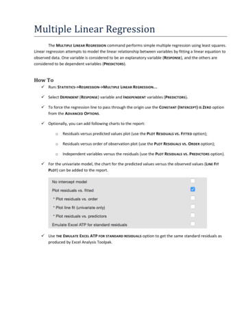
Multiple Linear RegressionThe MULTIPLE LINEAR REGRESSION command performs simple multiple regression using least squares.Linear regression attempts to model the linear relationship between variables by fitting a linear equation toobserved data. One variable is considered to be an explanatory variable (RESPONSE ), and the others areconsidered to be dependent variables (PREDICTORS).How To Run: STATISTICS- REGRESSION- MULTIPLE LINEAR REGRESSION. Select DEPENDENT (RESPONSE ) variable and INDEPENDENT variables (PREDICTORS). To force the regression line to pass through the origin use the CONSTANT (INTERCEPT) IS ZERO optionfrom the ADVANCED OPTIONS. Optionally, you can add following charts to the report:oResiduals versus predicted values plot (use the PLOT RESIDUALS VS. FITTED option);oResiduals versus order of observation plot (use the PLOT RESIDUALS VS. ORDER option);oIndependent variables versus the residuals (use the PLOT RESIDUALS VS. PREDICTORS option). For the univariate model, the chart for the predicted values versus the observed values (LINE FITPLOT) can be added to the report. Use THE EMULATE EXCEL ATP FOR STANDARD RESIDUALS option to get the same standard residuals asproduced by Excel Analysis Toolpak.

ResultsRegression statistics, analysis of variance table, coefficients table and residuals report are produced.Regression StatisticsR2 (COEFFICIENT OF DETERMINATION, R-SQUARED) is the square of the sample correlation coefficient betweenthe PREDICTORS (independent variables) and RESPONSE (dependent variable). In general, R2 is a percentageof response variable variation that is explained by its relationship with one or more predictor variables.In simple words, the R2 indicates the accuracy of the prediction. The larger the R2 is, the more the totalvariation of RESPONSE is explained by predictors or factors in the model. The definition of the R2 is𝑆𝑆𝑅 2 1 𝑆𝑆𝑒𝑟𝑟𝑜𝑟 .𝑡𝑜𝑡𝑎𝑙ADJUSTED R2 (ADJUSTED R-SQUARED) is a modification of R2 that adjusts for the number of explanatory termsin a model. While R2 increases when extra explanatory variables are added to the model, the adjusted R2increases only if the added term is a relevant one. It could be useful for comparing the models with differentnumbers of predictors. Adjusted R2 is computed using the formula:𝑆𝑆𝑑𝑓𝑁 1𝐴𝑑𝑗𝑢𝑠𝑡𝑒𝑑 𝑅 2 1 𝑆𝑆𝑒𝑟𝑟𝑜𝑟 𝑑𝑓𝑡𝑜𝑡𝑎𝑙 1 (1 𝑅 2 ) 𝑁 𝑘 1, where k is the number of excluding the intercept. Negative values (truncated to 0) suggest explanatory variables insignificance, oftenthe results may be improved by increasing the sample size or avoiding correlated predictors.MSE – the mean square of the error, calculated by dividing the sum of squares for the error term (residual)by the degrees of freedom (𝑑𝑓𝑒𝑟𝑟𝑜𝑟 𝑛 𝑝, 𝑝 is the number of terms).RMSE (root-mean-square error) – the estimated standard deviation of the error in the model. Calculated asthe square root of the MSE.PRESS – the squared sum of the PRESS residuals, defined in the RESIDUALS AND REGRESSION DIAGNOSTICS.PRESS RMSE is defined as 𝑃𝑅𝐸𝑆𝑆/𝑁. Provided for comparison with RMSE.2PREDICTED R-SQUARED is defined as 𝑅𝑃𝑟𝑒𝑑 1 𝑃𝑅𝐸𝑆𝑆/𝑆𝑆𝑇𝑜𝑡𝑎𝑙 . Negative values indicate that the PRESS isgreater than the total SS and can suggest the PRESS inflated by outliers or model overfitting. Some appstruncate negative values to 0.TOTAL NUMBER OF OBSERVATIONS N - the number of observations used in the regression analysis.The REGRESSION EQUATION takes the form Y 𝑎1 𝑥1 𝑎2 𝑥2 𝑎𝑘 𝑥𝑘 c 𝑒, where Y is thedependent variable and the a's are the regression coefficients for the corresponding independent terms 𝑥𝑖(or slopes), c is the constant or intercept, and e is the error term reflected in the residuals. Regressionequation with no interaction effects is often called main effects model.When there is a single explanatory variable the regression equation takes the form of equation of thestraight line: Y a 𝑥 c. Coefficient 𝑎 is called a slope and c is called an intercept. For this simple casethe slope is equal to the correlation coefficient between Y and 𝑥 corrected by the ratio of standarddeviations.Analysis of Variance TableSOURCE OF VARIATION - the source of variation (term in the model). The TOTAL variance is partitioned intothe variance, which can be explained by the independent variables (REGRESSION), and the variance, which isnot explained by the independent variables (ERROR, sometimes called RESIDUAL ).SS (SUM OF SQUARES) - the sum of squares for the term.

DF (DEGREES OF FREEDOM ) - the number of observations for the corresponding model term. The TOTALvariance has N – 1 degrees of freedom. The REGRESSION degrees of freedom correspond to the number ofcoefficients estimated, including the intercept, minus 1.MS (MEAN SQUARE) - an estimate of the variation accounted for by this term. 𝑀𝑆 𝑆𝑆/𝐷𝐹F - the F-test statistic.P-VALUE - p-value for a F-test. A value less than 𝛼 level shows that the model estimated by the regressionprocedure is significant.Coefficient EstimatesCOEFFICIENTS - the values for the regression equation.STANDARD ERROR - the standard errors associated with the coefficients.LCL, UCL are the lower and upper confidence intervals for the coefficients, respectively. Default 𝛼 level canbe changed in the PREFERENCES.T STAT - the t-statistics, used to test whether a given coefficient is significantly different from zero.P-VALUE - p-values for the alternative hypothesis (coefficient differs from 0). A low p-value (p 0.05) allowsthe null hypothesis to be rejected and means that the variable significantly improves the fit of the model.VIF – variance inflation factor, measures the inflation in the variances of the parameter estimates due tocollinearities among the predictors. It is used to detect multicollinearity problems. The larger the value is,the stronger the linear relationship between the predictor and remaining predictors.VIF equal to 1 indicates the absence of a linear relationship with other predictors (there is nomulticollinearity). VIF value between 1 and 5 indicates moderate multicollinearity, and values greater than 5suggest that a high degree of multicollinearity is present. It is a subject of debate whether there is a formalvalue for determining the presence of multicollinearity: in some situations even values greater than 10 canbe safely ignored – when high values caused by complicated models with dummy variables or variables thatare powers of other variables. In weaker models even values above 2 or 3 may be a cause for concern: forexample, for ecological studies Zuur, et al. (2010) recommended a threshold of VIF 3.TOL - the tolerance value for the parameter estimates, it is defined as TOL 1 / VIF.

Residuals and Regression DiagnosticsPREDICTED values or fitted values are the values that the model predicts for each case using the regressionequation.RESIDUALS are differences between the observed values and the corresponding predicted values. Residualsrepresent the variance that is not explained by the model. The better the fit of the model, the smaller thevalues of residuals. Residuals are computed using the formula:𝑒𝑖 𝑂𝑏𝑠𝑒𝑟𝑣𝑒𝑑 𝑣𝑎𝑙𝑢𝑒 𝑃𝑟𝑒𝑑𝑖𝑐𝑡𝑒𝑑 𝑣𝑎𝑙𝑢𝑒 𝑦𝑖 𝑦̂𝑖 .Both the sum and the mean of the residuals are equal to zero.STANDARDIZED residuals are the residuals divided by the square root of the variance function. Standardizedresidual is a z-score (standard score) for the residual. Standardized residuals are also known as standardresiduals, semistudentized residuals or Pearson residuals (ZRESID). Standardized and studentized residualsare useful for detection of outliers and influential points in regression. Standardized residuals are computedwith the untenable assumption of equal variance for all residuals.𝑒𝑖𝑒𝑖𝑒𝑠𝑖 𝑠 𝑀𝑆𝐸MSE is the mean squared-error of the model.STUDENTIZED residuals are the internally studentized residuals (SRESID). The internally studentized residual isthe residual divided by its standard deviation. The t-score (Student’s t-statistic) is used for residualsnormalization. The internally studentized residual 𝑟𝑖 is calculated as shown below (ℎ̃𝑖 is the leverage of theith observation).𝑒𝑖𝑒𝑖𝑟𝑖 𝑠(𝑒𝑖 ) 𝑀𝑆𝐸(1 ℎ̃𝑖 )DELETED T – studentized deleted residuals or externally studentized residuals (SDRESID), are oftenconsidered to be more effective for detecting outlying observations than the internally studentizedresiduals or Pearson residuals. A rule of thumb is that observations with an absolute value larger than 3 areoutliers (Hubert, 2004). Please note that some software packages report the studentized deleted residualsas simply “studentized residuals”.Externally studentized residual 𝑡𝑖 (deleted t residual) is defined as the deleted residual divided by itsestimated standard deviation.𝑡𝑖 𝑑𝑖 𝑠(𝑑𝑖 )𝑒𝑖𝑛 𝑝 1 𝑒𝑖 𝑀𝑆𝐸(1 ℎ̃𝑖 ) 𝑒𝑖 2 𝑀𝑆𝐸𝑖 (1 ℎ̃𝑖 )p is the number of terms (the number of regression parameters including the intercept).thThe deleted residual is defined as 𝑑𝑖 𝑦𝑖 𝑦̂(𝑖) , where 𝑦̂(𝑖) is the predicted response for the i observationbased on the model with the ith observation excluded. The mean square error for the model with the ithobservation excluded (𝑀𝑆𝐸𝑖 ) is computed from the following equation:(𝑛 𝑝)𝑀𝑆𝐸 (𝑛 𝑝 1)𝑀𝑆𝐸𝑖 𝑒𝑖 2 /(1 ℎ̃𝑖 ).LEVERAGE ℎ̃𝑖 is a measure of how much influence each observation has on the model. Leverage of the ithobservation can be calculated as the ith diagonal element of the hat matrix 𝐻 𝑋(𝑋 𝑇 𝑋) 1 𝑋 𝑇 . Leveragevalues range from 0 (an observation has no influence) to 1 (an observation has complete influence over̅ 𝑝/𝑛.prediction) with average value of ℎ̃𝑖

Stevens (2002) suggests to carefully examine unusual observations with a leverage value greater than 3𝑝/𝑛.Huber (2004) considers observations with values between 0.2 and 0.5 as risky and recommends to avoidvalues above 0.5.COOK'S D – Cook's distance, is a measure of the joint (overall) influence of an observation being an outlier onthe response and predictors. Cook’s distance expresses the changes in fitted values when an observation isexcluded and combines the information of the leverage and the residual. Values greater than 1 are generallyconsidered large (Cook and Weisberg, 1982) and the corresponding observations can be influential. It iscalculated as:𝑒𝑖 2ℎ̃𝑖𝐷𝑖 .𝑝 𝑀𝑆𝐸 (1 ℎ̃𝑖 )2DFIT or DFFITS (abbr. difference in fits) – is another measure of the influence. It combines the informationof the leverage and the studentized deleted residual (deleted t) of an observation. DFIT indicates the changeof fitted value in terms of estimated standard errors when the observation is excluded. If the absolute valueis greater than 2 𝑝/(𝑛 𝑝) 2 𝑝/𝑛, the observation is considered as an influential outlier (Belsley, Kuhand Welsch, 1980).ℎ̃𝑖𝐷𝐹𝐼𝑇𝑖 𝑡𝑖 1 ℎ̃𝑖PRESS (predicted residual error sum of squares) residual or prediction error is simply a deleted residualdefined above. The smaller the 𝑑𝑖 value is, the better the predictive power of the model. The squared sumof the deleted residuals (PRESS residuals) is known as the PRESS statistic: 𝑃𝑅𝐸𝑆𝑆 𝑑𝑖 2 .