WIXLIB

Quantitative Literacy Across the CurriculumImproving Graphs in College TextbooksNaomi B. Robbins, Ph.D. and Joyce Robbins, Ph.D.Visual Business Intelligence NewsletterFebruary 2010IntroductionThis newsletter is well known for its criticism of the graphs produced by many Business Intelligence (BI)software vendors. This criticism is well-deserved. In this issue we examine an equally disturbing source ofconfusing and misleading graphs: those found in introductory college social science textbooks. Given theimportance of statistics to the social sciences and the prevalence of social science requirements, it’s fair toassume that introductory courses significantly influence students’ understanding of data presentation. Wewould expect that the wealth of graphs in social science textbooks would conform to the highest standards ofdata presentation principles.What one finds in these textbooks, however, is often disappointing. While the quality does vary amongtextbooks, a surprising number include graphs which contain all kinds of distortions due to poor graphingtechniques. Furthermore, we have found that the same bad graphs appear in edition after edition of thesebooks; the popular social science textbooks today tend to come out with a new edition on a very frequent basis.Not only do students miss substantively what the graph attempts to communicate, but they learn inappropriatemethods for displaying data visually. In this article, we provide examples and describe in detail some errorsfound using pie, bar and line charts as well as tables. It is our hope that by drawing attention to this situation wecan begin the process of correcting the problem. Although there are problems with the graphs in many texts,we will single out one textbook that contains more than its share of distorted graphs: Introduction to Sociologyby Henry Tischler.Graph forms covered: a short disclaimerPie charts, bar charts, line graphs, and tables are among the most common forms of communicating numbers,and not surprisingly, they are the most common forms found in social science textbooks. This in itself isproblematic, since many data presentation experts recommend against overuse of pie charts and bar charts.In our view, pie charts do not communicate data well and should be used rarely. (For more information onproblems with pie charts, see Becker and Cleveland [1], Tufte [11], Robbins [5], and Few [4].) Bar charts aremore controversial. Cleveland [2] recommends dot plots instead of bar charts. Tufte [11] criticizes bar chartssince they have high redundancy with a low data-ink ratio. Following Cleveland, we do not recommend usingbar charts with error bars, logarithmic scales, or when zero is not included in the scale. We find that bar chartsget cluttered quickly while dot plots do not. We are more open to the use of bar charts for very small datasets. Properly drawn line graphs tend to communicate numerical data well. Tables are extremely useful whenprecision is needed but the design of most tables could be improved.That said, for the purpose of this critique, we take the position that whatever form is chosen, it should beexecuted properly. Therefore, rather than take aim at forms that we think are less effective and promote thosethat are more effective, we point out problems within the chosen graph genre.In short, whether we like it or not, these graph forms are widely known and used and are likely to continue tobe used frequently. Therefore, they should be designed to communicate numerical data as clearly as possible.Line graphs are less likely to have errors than pie and bar charts, yet we find many design flaws with this formas well. In the following sections we point out errors that distort the data in a number of graphs.Copyright 2010 Naomi B. Robbins and Joyce RobbinsPage 1 of 7

Pie ChartsFigure 1. Pie charts do not communicate information well. The added pseudo-third dimension and tiltedcircle shown above make the problem worse.Adding a pseudo-third dimension distorts the data, emphasizing some wedges at the expense of others.Adding perspective or tilting the bar distorts the data even more.A graph is a pictorial representation of numbers. At the least, the elements of the graph representing thenumbers should be proportional to the numbers themselves. The percentages in a pie chart are representedby the angles of the wedges, the areas of the wedges, or the arc lengths of the wedges. To our eyes, the angleof the “Organized child-care facility” wedge looks much smaller than the “Care in another home” wedge, eventhough the values in the labels are close (29.3% vs. 31.3%). Tilting and elongating the pie is poor graphicalpractice and does not belong in an introductory text. Interestingly enough, the previous edition of this text useda simple two-dimensional pie chart for similar data. Although software packages increasingly offer elaboratedesign options, in most cases, for communicating data, less is more.Bar ChartsFigure 2. Most readers will not know how to read these charts; the slanted ends are confusing.Copyright 2010 Naomi B. Robbins and Joyce RobbinsPage 2 of 7

The numbers in a bar chart are represented by the length of the bar or the position of the end of the bar.Neither is clear with the bars of Figure 2 because the ends of the bars slant.Notice that the “average time actually served” for drug possession is ten months and ten is one of the labelson the horizontal scale. However, since there are no tick marks, we cannot tell exactly where ten falls on thescale. Both the top and bottom of the end of that bar appear larger than the midpoint of the label “10”. Graphsshould communicate quantitative information rather than confuse readers and make them do detective work todecipher the information.Figure 3. This figure also suffers from slanted bar ends and is deceptive since thejudgment of lengths requires a zero base.The bar chart in Figure 3 is more confusing since, in addition to the slanted ends of the bars, the chart ismissing a zero baseline. This is crucial since we judge the values of bars by their lengths and lengths requirea zero base. Without zero the comparison is deceptive. Even if you think you are comparing the bars by theposition of their endpoints, you cannot help but notice the lengths of the bars as well. For example, the lengthof the bar for “high school graduate” looks about triple that for “high school dropout” but based on the tickmarks, both are between 500 and 1000.Figure 4.The slanting bars and frame for this graph only serve to confuse. Furthermore,the reader can’t tell whether each bar is associated with a decade or year, and if thelatter, whether the label is to the right or left of the bar.Copyright 2010 Naomi B. Robbins and Joyce RobbinsPage 3 of 7

The ends of the bars slanted in Figures 2 and 3; here the whole bar slants. This serves no purpose other thanto confuse the reader. Comparing the heights of the first two bars shows that the figure is not drawn to scale:the height of the “0.6” bar should be six times the height of the “0.1” bar which it clearly is not.In addition, it is not clear if the values of the bars represent immigration for the years labeled or for decades.If it is years, it is not clear which label is associated with each bar since there are 20 labels and 19 bars. (It iseasy to determine that there are more labels than bars by noting that there is a label to the left of the first barand also one to the right of the last bar.) However, we know from other sources that the data correspond toimmigration by decade. (See Dinnerstein et al. [3] for an excellent graph of the same data.) This is impossibleto determine from this figure.Another problem with Figure 4 is that it suggests that immigration decreased after 2000. However, the final barrepresents four years while the others represent ten years, and therefore the short bar is deceptive.Line GraphsFigure 5. This figure distorts the data by using evenly spaced tick mark labels for unequal intervals.This figure shows the number of prisoners sentenced to death from 1953 through 2004, a period of just over 50years. The data from 1953 to 1994 (over a forty year span) takes up less than half of the horizontal axis whilethe remaining eleven years takes over half. The labels from 1994 to 2004 are evenly spaced but do not allrepresent the same intervals of time: from 1994 to 1999 the interval represents one year, then the next intervalrepresents two years and the final one three years. On the vertical axis we have evenly spaced gridlines thatbegin at intervals of 500 prisoners. We see 0, 500, 1000, 1500, 2000, and then 2356. Evenly spaced tick marksshould represent the same intervals when using a linear scale.Copyright 2010 Naomi B. Robbins and Joyce RobbinsPage 4 of 7

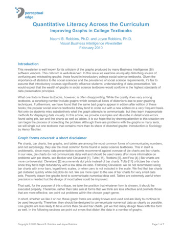
The footnote in the figure shows that the source of the data is the US Department of Justice. We were curiousto see how they presented these data so we went to their Web site and found the following figure.Figure 6. This figure, showing the same data as Figure 5, appears on theDepartment of Justice Web page.Notice that the horizontal axis is labeled at five year intervals and the vertical axis at 500 prisoners, so thatthis figure is drawn to scale. We’d prefer that the horizontal axis had tick marks so we could tell more preciselywhere each year fell, but this is very minor next to the distortions of Figure 5. If we compare the two figureswe notice that the percentage of the time axis with a relatively low number of prisoners on death row is muchlarger in Figure 6 than in Figure 5. We also notice the differences of the rate of increase. The big bulge inFigure 5 does not appear in Figure 6.Figure 7. Here all the labels are ten years apart but the tick marks are not equally spaced.In Figure 5 the labels did not represent even intervals while in Figure 7 the labels do represent even intervalsbut their distribution over the axis is not even. The end result is the same: a distortion of the data.Copyright 2010 Naomi B. Robbins and Joyce RobbinsPage 5 of 7