Transcription
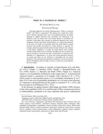
The Annals of Statistics2002, Vol. 30, No. 5, 1225–1310WHAT IS A STATISTICAL MODEL?1B Y P ETER M C C ULLAGHUniversity of ChicagoThis paper addresses two closely related questions, “What is a statisticalmodel?” and “What is a parameter?” The notions that a model must “makesense,” and that a parameter must “have a well-defined meaning” are deeplyingrained in applied statistical work, reasonably well understood at aninstinctive level, but absent from most formal theories of modelling andinference. In this paper, these concepts are defined in algebraic terms, usingmorphisms, functors and natural transformations. It is argued that inferenceon the basis of a model is not possible unless the model admits a naturalextension that includes the domain for which inference is required. Forexample, prediction requires that the domain include all future units, subjectsor time points. Although it is usually not made explicit, every sensiblestatistical model admits such an extension. Examples are given to show whysuch an extension is necessary and why a formal theory is required. In thedefinition of a subparameter, it is shown that certain parameter functionsare natural and others are not. Inference is meaningful only for naturalparameters. This distinction has important consequences for the constructionof prior distributions and also helps to resolve a controversy concerning theBox–Cox model.1. Introduction. According to currently accepted theories [Cox and Hinkley (1974), Chapter 1; Lehmann (1983), Chapter 1; Barndorff-Nielsen andCox (1994), Section 1.1; Bernardo and Smith (1994), Chapter 4] a statisticalmodel is a set of probability distributions on the sample space S. A parameterizedstatistical model is a parameter set together with a function P : P (S),which assigns to each parameter point θ a probability distribution Pθ on S.Here P (S) is the set of all probability distributions on S. In much of the following,it is important to distinguish between the model as a function P : P (S), andthe associated set of distributions P P (S).In the literature on applied statistics [McCullagh and Nelder (1989); Gelman,Carlin, Stern and Rubin (1995); Cox and Wermuth (1996)], sound practical adviceis understandably considered to be more important than precise mathematicalReceived January 2000; revised July 2001.1 Supported in part by NSF Grants DMS-97-05347 and DMS-00-71726.AMS 2000 subject classifications. Primary 62A05; secondary 62F99.Key words and phrases. Aggregation, agricultural field experiment, Bayes inference, Box–Coxmodel, category, causal inference, commutative diagram, conformal model, contingency table,embedding, exchangeability, extendability, extensive variable, fertility effect, functor, Gibbs model,harmonic model, intensive variable, interference, Kolmogorov consistency, lattice process, measureprocess, morphism, natural parameterization, natural subparameter, opposite category, quadraticexponential model, representation, spatial process, spline model, type III model.1225
1226P. MCCULLAGHdefinitions. Thus, most authors do not offer a precise mathematical definition ofa statistical model. Typically, the preceding definition is taken for granted, andapplied to a range of sensibly constructed models.At a minimum, a Bayesian model requires an additional component in theform of a prior distribution on . A Bayesian model in the sense of Berger(1985), Smith (1984) or Bernardo and Smith (1994) requires an extra componentin the form of a judgment of infinite exchangeability or partial exchangeabilityin which parameters are defined by limits of certain statistics. Although Bayesianformulations are not the primary focus of this paper, the notion that the model isextendable to a sequence, usually infinite, is a key concept.The parameterization is said to be identifiable if distinct parameter valuesgive rise to distinct distributions; that is, Pθ Pθ implies θ θ . Thus, theparameter is identifiable if and only if P : P (S) is injective. Apart fromthese conditions, the standard definition permits arbitrary families of distributionsto serve as statistical models, and arbitrary sets to serve as parameter spaces.For applied work, the inadequacy of the standard definition is matched only bythe eccentricity of the formulations that are permitted. These examples make itabundantly clear that, unless the model is embedded in a suitable structure thatpermits extrapolation, no useful inference is possible, either Bayesian or nonBayesian.To be fair, most authors sound a note of warning in their discussion ofstatistical models. Thus, for example, Cox and Hinkley [(1974), Chapter 1], whileadmitting that “it is hard to lay down precise rules for the choice of the familyof models,” go on to offer a range of recommendations concerning the modeland the parameterization. In particular, “the model should be consistent withknown limiting behavior” and the parameterization should be such that “differentparameter [components] have individually clear-cut interpretations.” The intentionof this article is to define some of these concepts in purely algebraic terms.2. Examples.2.1. Twelve statistical exercises. The following list begins with four exercisesin which the models are plainly absurd. The point of the exercises, however, is notso much the detection of absurd models as understanding the sources of absurdity.From a more practical viewpoint, the more interesting exercises are those in whichthe absurdity is not obvious at first sight.E XERCISE 1 (A binary regression model). Consider a model for independentbinary responses in which certain covariates are prespecified. One of thesecovariates is designated the treatment indicator. The model specifies a logit linkif the number of subjects is even, and a probit link otherwise. Inference is requiredfor the treatment effect. Predictions are required for the response of a future subjectwith specified covariate values.
WHAT IS A STATISTICAL MODEL?1227E XERCISE 2 (A randomized blocks model). Consider a randomized blocksdesign with b blocks and k varieties. In the statistical model, all observations areindependent and normally distributed with unit variance. The expected yield µijof variety i in block j is assumed to be expressible in the following manner forsome real-valued function α on varieties and β on blocks: µij αi βj ,exp(αi βj ),if k b is even,otherwise.On the basis of this model, inference is required in the form of a confidence intervalor posterior distribution for a particular variety contrast α1 α2 .E XERCISE 3 (A linear regression model). In the standard linear regressionmodel Y N (Xβ, σ 2 In ) on Rn , the parameter (β, σ 2 ), is a point in Rp [0, ).In our modified eccentric version, the parameter space is Rp [n, ), sothat σ 2 n. A prediction interval is required for the value of the response on anew subject whose covariate value is x Rp .E XERCISE 4 [An i.i.d. normal model (Section 6.6)]. In this model, theobservations are independent, identically distributed and normal. The parameterspace is R2 . If n is even, the mean is θ1 and the variance is θ22 : otherwise, themean is θ2 and the variance is θ12 . On the basis of observed values (y1 , . . . , yn ),inference is required in the form of confidence limits or a posterior distributionon .E XERCISE 5 [The type III model (Section 6.6)]. Consider a randomizedblocks design as in Exercise 2 above, all observations being independent, normalwith unit variance. According to the type III model as described in the SAS manual[Littell, Freund and Spector (1991), pages 156–160], the vector µ lies in the linearsubspace III kb of dimension bk k 1 such that the k variety means are equal,III kb {µ Rkb : µ̄1. · · · µ̄k. }.On the assumption that the fit is adequate, what conclusions can be drawn aboutvariety differences on either a subset of the blocks or on other blocks similar tosome of those used in the experiment?E XERCISE 6 [The Box–Cox model (Section 7)]. In the Box–Cox model[Box and Cox (1964)], it is assumed that after some componentwise powertransformation Yi Yiλ , the transformed response variable satisfies the standardnormal-theory linear model with mean E(Y λ ) Xβ and constant variance σ 2 .In the problem posed by Bickel and Doksum (1981), inference is required in theform of confidence intervals or a posterior distribution for the parameter β or acomponent thereof.
1228P. MCCULLAGHE XERCISE 7 [A model for clustered data (Section 6.6)]. In a cluster ofsize k, the response Y has joint density with respect to Lebesgue measure on Rkproportional to 1 2 1 yi yjexp θ1yi θ222 i j k 1 for some θ1 0 and 0 θ2 θ1 . Thus, the vector Y is normally distributed withzero mean and exchangeable components. Observations on distinct clusters areindependent. On the basis of the observed data (k1 , Y1 ), . . . , (kn , Yn ), in whichkr is the size of cluster r and Yr normally distributed on Rkr , a confidence set isrequired for θ . In particular, if the observed clusters are all of size 2, inference isrequired for the distribution of the cluster mean in a cluster of size 8.E XERCISE 8 [An i.i.d. Cauchy model (Section 6.6)]. By the two-parameterCauchy family is meant the set of distributions on R with densities θ2 dy: θ2 0, θ1 R .2π(θ2 (y θ1 )2 )Let Y1 , . . . , Yn be n independent and identically distributed random variables withdistribution in the two-parameter Cauchy family. A confidence interval or posteriordistribution is required for the parameter θ1 . The catch here is that the Cauchyfamily is closed under the real fractional linear group, and the confidence intervalis required to have the corresponding property. In other words, for any real numbersa, b, c, d such that ad bc 0, the random variables Zi (aYi b)/(cYi d)are i.i.d. Cauchy. If we write θ θ1 iθ2 as a conjugate pair of complex numbers,the transformed parameter is ψ (aθ b)/(cθ d) [McCullagh (1992, 1996)].The procedure used must be such that if the values Z1 , . . . , Zn are reported as i.i.d.Cauchy(ψ), and a confidence interval is requested for θ1 ((dψ b)/(a cψ)),the same answer must be obtained regardless of the values a, b, c, d.E XERCISE 9 (A model for a spatial process). The temperature in a roomis modelled as a stationary isotropic Gaussian process in which the meantemperature is constant E(Yx ) µ, and the covariance function is cov(Yx , Yx ) σ 2 exp( λ x x ). The parameter space is(µ, σ 2 , λ) R (0, )2 .A confidence interval is required for θ µ/σ .E XERCISE 10 [Regression and correlation (Section 6.2)]. Consider thestandard normal-theory linear regression model with one covariate in which
WHAT IS A STATISTICAL MODEL?1229the observations are independent, normally distributed with conditional meanE(Y x) α βx and constant variance σ 2 . The parameter space is(α, β, σ 2 ) R2 [0, ).A confidence interval or posterior distribution is required for the correlationcoefficient.E XERCISE 11 [Spatial simultaneous equation model (Section 6.5)]. Let Y bea spatial process observed on a rectangular lattice of sites. The joint distribution isdefined by a set of simultaneous equationsYi βYj εi ,j iin which j i means that site j i is a neighbour of site i. This expression isinterpreted to mean that (I B)Y ε is standard normal. The components of Bare zero except for neighboring sites for which bij β. The system is such thatI B is invertible, so that Y is normal with zero mean and inverse covariancematrix (I B)T (I B). A confidence interval is required for β.E XERCISE 12 [Contingency table model (Section 6.4)]. All three factors ina contingency table are responses. In principle, each factor has an unboundednumber of levels, but some aggregation has occurred, and factor B is in factrecorded in binary form. The log-linear model AB BC is found to fit well, butno log-linear submodel fits. What conclusions can be drawn?2.2. Remarks. These exercises are not intended to be comparable in theirdegree of absurdity. They are intended to illustrate a range of model formulationsand inferential questions, some clearly artificial, some a little fishy, and othersbordering on acceptability. In the artificial class, I include Exercises 1, 2, 4,and possibly 3. Exercise 9 ought also to be regarded as artificial or meaninglesson the grounds of common sense. The type III model has been criticized froma scientific angle by Nelder (1977) in that it represents a hypothesis of noscientific interest. Despite this, the type III model continues to be promoted in textbooks [Yandell (1997), page 172] and similar models obeying the so-called weakheredity principle [Hamada and Wu (1992)] are used in industrial experiments.The absurdity in the other exercises is perhaps less obvious. Although they appearradically different, from an algebraic perspective Exercises 2 and 5 are absurd inrather similar ways.Each of the formulations satisfies the standard definition of a statistical model.With respect to a narrowly defined inferential universe, each formulation isalso a statistical model in the sense of the definition in Sections 1 and 4.Inference, however, is concerned with natural extension, and the absurdity of
1230P. MCCULLAGHeach formulation lies in the extent of the inferential universe or the scope of themodel. Although a likelihood function is available in each case, and a posteriordistribution can be computed, no inferential statement can breach the bounds of theinferential universe. To the extent that the scope of the model is excessively narrow,none of the formulations permits inference in the sense that one might reasonablyexpect. We conclude that, in the absence of a suitable extension, a likelihood anda prior are not sufficient to permit inference in any commonly understood sense.3. Statistical models.3.1. Experiments. Each statistical experiment or observational study is builtfrom the following objects:1. A set U of statistical units, also called experimental units, plots, or subjects;2. A covariate space );3. A response scale V.The design is a function x : U ) that associates with each statistical uniti U a point xi in the covariate space ). The set D )U of all such functionsfrom the units into the covariate space is called the design space.The response is a function y : U V that associates with each statistical unit i,a response value yi in V. The set S V U of all such functions is called thesample space for the experiment. In the definition given in Section 1, a statisticalmodel consists of a design x : U ), a sample space S V U and a family ofdistributions on S.A statistical model P : P (S) associates with each parameter value θa distribution P θ on S. Of necessity, this map depends on the design, for example,on the association of units with treatments, and the number of treatment levels thatoccur. Thus, to each design x : U ), there corresponds a map Px : P (S)such that Px θ is a probability distribution on S. Exercise 2 suggests strongly thatthe dependence of Px on x D cannot be arbitrary or capricious.3.2. The inferential universe. Consider an agricultural variety trial in whichthe experimental region is a regular 6 10 grid of 60 rectangular plots, eachseven meters by five meters, in which the long side has an east–west orientation.It is invariably understood, though seldom stated explicitly, that the purpose ofsuch a trial is to draw conclusions concerning variety differences, not just forplots of this particular shape, size and orientation, but for comparable plots ofvarious shapes, sizes and orientations. Likewise, if the trial includes seven potatovarieties, it should ordinarily be possible to draw conclusions about a subset ofthree varieties from the subexperiment in which the remaining four varieties areignored. These introductory remarks may seem obvious and unnecessary, but theyhave far-reaching implications for the construction of statistical models.
WHAT IS A STATISTICAL MODEL?1231The first point is that before any model can be discussed it is necessary toestablish an inferential universe. The mathematical universe of experimental unitsmight be defined as a regular 6 10 grid of 7 5 plots with an east–westorientation. Alternatively, it could be defined as the set of all regular grids ofrectangular plots, with an east–west orientation. Finally, and more usefully, theuniverse could be defined as a suitably large class of subsets of the plane, regardlessof size, shape and orientation. From a purely mathematical perspective, each ofthese choices is internally perfectly consistent. From the viewpoint of inference,statistical or otherwise, the first and second choices determine a limited universe inwhich all inferential statements concerning the likely yields on odd-shaped plotsof arbitrary size are out of reach.In addition to the inferential universe of statistical units, there is a universeof response scales. In an agricultural variety trial, the available interchangeableresponse scales might be bushels per acre, tones per hectare, kg/m2 , and so on.In a physics or chemistry experiment, the response scales might be C, K, F,or other suitable temperature scale. In a food-tasting experiment, a seven-pointordered scale might be used in which the levels are labelled asV {unacceptable, mediocre, . . . , excellent},or a three-point scale with levelsV {unacceptable, satisfactory, very good}.It is then necessary to consider transformations V V in which certain levelsof V are, in effect, aggregated to form a three-level scale. Finally, if the responsescale is bivariate, including both yield and quality, this should not usually precludeinferential statements concerning quality or quantity in isolation.Similar comments are in order regarding the covariate space. If, in theexperiment actually conducted, fertilizer was applied at the rates, 0, 100, 200 and300 kg/ha, the inferential universe should usually include all nonnegative doses.Likewise, if seven varieties of potato were tested, the inferential universe shouldinclude all sets of varieties because these particular varieties are a subset of othersets of varieties. This does not mean that informative statements can be made aboutthe likely yield for an unobserved variety, but it does mean that the experimentperformed may be regarded as a subset of a larger notional experiment in whichfurther varieties were tested but not reported.3.3. Categories. Every logically defensible statistical model in the classicalsense has a natural extension from the set of observed units, or observed varieties,or observed dose levels, to other unobserved units, unobserved blocks, unobservedtreatments, unobserved covariate values and so on. Thus, in constructing astatistical model, it is essential to consider not only the observed units, the observedblocks, the observed treatments and so on, but the inferential universe of all
1232P. MCCULLAGHrelevant sample spaces, all relevant sets of blocks, all relevant covariate valuesand so on. Every sensible statistical model does so implicitly. The thesis of thispaper is that the logic of every statistical model is founded, implicitly or explicitly,on categories of morphisms of the relevant spaces. The purpose of a category isto ensure that the families of distributions on different sample spaces are logicallyrelated to one another and to ensure that the meaning of a parameter is retainedfrom one family to another.A category C is a set of objects, together with a collection of arrows representingmaps or morphisms between pairs of objects. In the simplest categories, eachobject is a set, and each morphism is a map. However, in the category of statisticaldesigns, each design is a map and each morphism is a pair of maps, so a morphismneed not be a map between sets. To each ordered pair (S, S ) of objects in C, therecorresponds a set homC (S, S ), also denoted by C(S, S ), of morphisms ϕ : S S ,with domain S and codomain S . For certain ordered pairs, this set may be empty.Two conditions are required in order that such a collection of objects and arrowsshould constitute a category. First, for each object S in C, the identity morphism1 : S S is included in hom(S, S). Second, for each pair of morphisms ϕ : S S and ψ : S S , such that dom ψ cod ϕ, the composition ψϕ : S S is amorphism in hom(S, S ) in C. In particular, the set hom(S, S) of morphismsof a given object is a monoid, a semigroup containing the identity and closedunder composition. A glossary of certain category terminology is provided in theAppendix. For all further details concerning categories, see Mac Lane (1998).In the discussion that follows, the symbol catU represents the category ofmorphisms of units. The objects in this category are all possible sets U, U , . . .of statistical units. These sets may have temporal, spatial or other structure.The morphisms ϕ : U U in catU are maps, certainly including all insertionmaps ϕ : U U (such that ϕu u) whenever U U . In general, catU is thecategory of morphisms that preserves the structure of the units, such as equivalencerelationships in a block design [McCullagh (2000), Section 9.5] or temporalstructure in time series. In typical regression problems therefore, catU is identifiedwith the the generic category I of injective, or 1–1, maps on finite sets. These arethe maps that preserve distinctness of units: u u in U implies ϕ(u) ϕ(u )in U .A response is a value taken from a certain set, or response scale. If the responseis a temperature, each object in catV is a temperature scale, including one objectfor each of the conventional scales C, F and K. To each ordered pair oftemperature scales (V, V ) there corresponds a single invertible map, which is anaffine transformation V V . Likewise, yield in a variety trial may be recordedon a number of scales such as bushels/acre, tones/ha or kg/m2 . To each responsescale there corresponds an object V in catV , and to each pair of response scalesthere corresponds a single invertible map, which is a positive scalar multiple. Fora typical qualitative response factor with ordered levels, the morphisms are orderpreserving surjections, which need not be invertible. Special applications call for
WHAT IS A STATISTICAL MODEL?1233other sorts of morphisms, such as censoring in survival data. The essential pointhere is that each response scale determines a distinct object in catV , and the mapsV V are surjective (onto).Since statistical inferences are invariably specific to the scale of measurement, itis absolutely essential that the various quantitative response scales not be fused intoone anonymous scale labelled R or R . An affine transformation of temperaturescales is a transformation ϕ : V V from one scale into another. Unless V V ,such a transformation is not composable with itself, a critical distinction that is lostif all scales are fused into R. Thus, although catV may be a category of invertiblemaps, it is ordinarily not a group.Likewise, the symbol cat) represents the category whose objects are thecovariate spaces, and whose morphisms are maps, ordinarily injective, betweencovariate spaces. Because of the great variety of covariate spaces, these maps aremore difficult to describe in general. Nonetheless, some typical examples can bedescribed.A quantitative covariate such as weight is recorded on a definite scale, such aspounds, stones or kg. To each scale ) there corresponds a set of real numbers,and to each pair (), ) ) of quantitative scales there corresponds a 1–1 map) ) , usually linear or affine. The objects in cat) are some or all subsetsof each measurement scale. For some purposes, it is sufficient to consider onlybounded intervals of each scale: for other purposes, all finite subsets may besufficient. Generally speaking, unless there is good reason to restrict the class ofsets, the objects in cat) are all subsets of all measurement scales. The morphismsare those generated by composition of subset insertion maps and measurementscale transformation. Thus, cat) may be such that there is no map from the set{ten stones, eleven stones} into {140 lbs, 150 lbs, 160 lbs} but there is one mapinto {x lbs : x 0} whose image is the subset {140 lbs, 154 lbs}.For a typical qualitative covariate such as variety with nominal unorderedlevels, the objects are all finite sets, and cat) may be identified with the genericcategory I, of injective maps on finite sets. If the levels are ordinal, cat) maybe identified with the subcategory of order-preserving injective maps. Factorialdesigns have several factors, in which case cat) is a category in which each objectis a product set ) )1 · · · )k . The relevant category of morphisms is usuallythe product category, one component category for each factor. For details, seeMcCullagh (2000).4. Functors and statistical models.4.1. Definitions. It is assumed in this section that the response is an intensivevariable, a V-valued function on the units. Extensive response variables arediscussed in Section 8. In mathematical terms, an intensive variable is a functionon the units: an extensive variable such as yield is an additive set function. Theimportance of this distinction in applied work is emphasized by Cox and Snell
1234P. MCCULLAGH[(1981), Section 2.1]. The implications for the theory of random processes arediscussed briefly by Kingman [(1984), page 235].In terms of its logical structure, each statistical model is constructed from thefollowing three components:1. A category catU in which each object U is a set of statistical units. Themorphisms U U in catU are all injective maps preserving the structureof the units. In typical regression problems, catU may be identified with thecategory I of all injective maps on finite sets.2. A category cat) in which each object ) is a covariate space. The morphisms) ) are all injective maps preserving the structure of the covariate spaces.3. A category catV in which each object V is a response scale. The morphismsV V are all maps preserving the structure of the response scale. These aretypically surjective.These three categories are the building blocks from which the design category,the sample space category and all statistical models are constructed.Given a set of units U and a covariate space ), the design is a map x : U )associating with each unit u U a point xu in the covariate space ). In practice,this information is usually coded numerically for the observed units in the formof a matrix X whose uth row is the coded version of xu . The set of all suchdesigns is a category catD in which each object x is a pair (U, )) together with amap x : U ). Since the domain and codomain are understood to be part of thedefinition of x, the set of designs is the set of all such maps with U in catU and) in cat) , in effect, the set of model matrices X with labelled rows and columns.Each morphism ϕ : x x in which x : U ) , may be associated with a pairof injective maps ϕd : U U in catU , and ϕc : ) ) in cat) such that thediagramxU U ϕd x ) ϕc ) commutes [Tjur (2000)]. In other words x ϕd and ϕc x represent the same designU ) . In matrix notation, X U XW in which U is a row selection matrix,and W is a code-transformation matrix.The general idea behind this construction can be understood by asking whatit means for one design to be embedded in another. Here we consider simpleembeddings obtained by selection of units or selection of covariate values. First,consider the effect of selecting a subset U U of the units and discarding theremainder. Let ϕd : U U be the insertion map that carries each u U to itselfas an element of U . The design that remains when the units not in U are discardedis the composition x ϕd : U ) , which is the restriction of x to U. The diagram
1235WHAT IS A STATISTICAL MODEL?may thus be completed by taking ) ) , ϕc the identity, and x x ϕd . Next,consider the effect of selection based on covariate values, that is, selecting onlythose units U whose covariate values lie in the subset ) ) . Let ϕc : ) ) and ϕd : U U be the associated insertion maps. The design map x : U ) isgiven by x restricted to the domain U and codomain ) ) . Finally, if U U ,) ) and ϕc is a permutation of ), the design ϕc x is simply the design x with arearrangement of labels. The same design could be obtained by suitably permutingthe units before using the design map x, that is, the design xϕd .4.2. Model. Let V be a fixed response scale. A response y on U is afunction y : U V, a point in the sample space V U . To each set U therecorresponds a sample space V U of V-valued functions on U. Likewise, to eachinjective morphism ϕ : U U in catU there corresponds a coordinate-projection map ϕ : V U V U . For f V U , the pullback map defined by functionalcomposition ϕ f f ϕ is a V-valued function on U. Thus (V, ) is a functoron catU , associating with each set U the sample space V U , and with each morphism ϕ : U U the map ϕ : V U V U by functional composition. Theidentity map U U is carried to the identity V U V U and the composite map ψϕ : U U to the composite ϕ ψ : V U V U in reverse order.Before presenting a general definition of a statistical model, it may be helpful togive a definition of a linear model. Let V be a vector space, so that the sample spaceV U is also a vector space. A linear model is a subspace of V U , suitably related tothe design. In the functor diagram below, each map in the right square is a linear transformation determined by functional composition. Thus, for f V ) , thepullback by ϕc is ϕc f f ϕc , which is a vector in V ) . Likewise, ψ f f ψ is a vector in V U ,DesignU ϕd U ψ ψ
Cox (1994), Section 1.1; Bernardo and Smith (1994), Chapter 4] a statistical model is a set of probability distributions on the sample spaceS. A parameterized statistical model is a parameter set together with a function P: P(S), which assigns to eac