Transcription
Chapter 2Load Flow Analysis2.1IntroductionLoad flow analysis is the most important and essential approach to investigatingproblems in power system operating and planning. Based on a specified generatingstate and transmission network structure, load flow analysis solves the steadyoperation state with node voltages and branch power flow in the power system.Load flow analysis can provide a balanced steady operation state of the powersystem, without considering system transient processes. Hence, the mathematicmodel of load flow problem is a nonlinear algebraic equation system withoutdifferential equations. Power system dynamic analysis (see Chaps. 5 and 6) investigates system stability under some given disturbances. Its mathematic modelincludes differential equations. It should be pointed out that dynamic analysis isbased on load flow analysis and the algorithm of load flow analysis is also the basefor dynamic analysis methods. Therefore, familiarity with the theory and algorithms of load flow analysis is essential to understanding the methodology ofmodern power system analysis.Using digital computers to calculate load flow started from the middle of the1950s. Since then, a variety of methods has been used in load flow calculation. Thedevelopment of these methods is mainly led by the basic requirements of load flowcalculation, which can be summed up as:1. The convergence properties2. The computing efficiency and memory requirements3. The convenience and flexibility of the implementationMathematically, the load flow problem is a problem of solving a system of nonlinearalgebraic equations. Its solution usually cannot avoid some iteration process. Thusreliable convergence becomes the prime criterion for a load flow calculation method. With the scale of power system continually expanding, the dimension of loadflow equations now becomes very high (several thousands to tens of thousands). Forthe equations with such high dimensions, we cannot ensure that any mathematicalmethod can converge to a correct solution. This situation requires the researchersand scholars in the power system analysis field to seek more reliable methods.X.‐F. Wang et al., Modern Power Systems Analysis.doi: 10.1007/978-0-387-72853-7, # Springer Science þ Business Media, LLC 200871
722 Load Flow AnalysisIn the early stages of using digital computers to solve power system load flowproblems, the widely used method was the Gauss–Seidel iterative method based ona nodal admittance matrix (it will be simply called the admittance method below)[4]. The principle of this method is rather simple and its memory requirement isrelatively small. These properties made it suit the level of computer and powersystem theory at that time. However, its convergence is not satisfactory. When thesystem scale becomes larger, the number of iteration increases sharply, and sometimes the iteration process cannot converge. This problem led to the use of thesequential substitution method based on the nodal impedance matrix (also calledthe impedance method).At the beginning of the 1960s, the digital computer had developed to the secondgeneration. The memory and computing speed of computers were improved significantly, providing suitable conditions for the application of the impedance method.As mentioned in Chap. 1, the impedance matrix is a full matrix. The impedancemethod requires the computer to store the impedance matrix that represents thetopology and parameters of the power network. Thus it needs a great amount ofcomputer memory. Furthermore, in each iteration, every element in the impedancematrix must be operated with, so the computing burden is very heavy.The impedance method improved convergence and solved some load flowproblems that the admittance method could not solve. Therefore, the impedancemethod was widely applied from then on and made a great contribution to powersystem design, operation, and research.The main disadvantage of the impedance method is its high memory requirement and computing burden. The larger the system is, the more serious thesedefects are. To overcome the disadvantage, the piecewise solution method basedon impedance matrix was developed [5]. This method divides a large system up intoseveral small local systems and only the impedance matrixes of local systems andthe impedances of tie lines between these local systems are to be stored in thecomputer. In this way, the memory requirement and computing burden are greatlyalleviated.The other approach to overcoming the disadvantages of the impedance method isto apply the Newton–Raphson method (also called the Newton method) [6]. TheNewton method is a typical method used to solve nonlinear equations in mathematics with very favorable convergence. As long as the sparsity of the Jacobean matrixis utilized in the iterative process, the computing efficiency of the Newton methodcan be greatly improved. Since the optimal order eliminating method [7] began tobe employed in the middle of the 1960s, the Newton method has surpassed theimpedance method in the aspects of convergence, memory demand, and computingspeed. It is still the favored method, and is widely used in load flow calculationtoday.Since the 1970s, the load flow calculating method continues to develop invarious ways. Among them the most successful is the fast decoupled method,also called the P Q decoupled method [8]. Comparing with the Newton method,this method is much simpler and more efficient algorithmically, and therefore morepopular in many applications.
2.2 Formulation of Load Flow Problem73In the recent 20 years, research on load flow calculation is still very active. Manycontributions seek to improve the convergence characteristics of the Newtonmethod and the P Q decoupled method [9–15]. Along with the development ofartificial intelligent theory, the genetic algorithm, artificial neural network algorithm, and fuzzy algorithm have also been introduced to load flow analysis [16–19].However, until now these new models and new algorithms still cannot replace theNewton method and P Q decoupled method. Because the scales of power systemscontinue to expand and the requirements for online calculation become more andmore urgent, the parallel computing algorithms are also studied intensively now andmay become an important research field [20].This chapter mainly discusses the currently widely used Newton method andP Q decoupled method.The degree of flexibility and convenience of load flow calculation are also veryimportant to computer application. In practice, load flow analysis is usually part ofan interactive environment, rather than a pure calculation problem. Therefore, thehuman–computer interface should be friendly, allowing users to monitor andcontrol the calculation process. To obtain an ideal operation scheme, it is usuallynecessary to modify the original data according to the computing results. Thus, thecomputing method should be flexible, permitting users to readily modify and adjusttheir operation scheme. Input and output processes should also receive carefulattention.Power system steady state analysis includes load flow analysis and static securityanalysis. Load flow analysis is mainly used in analyzing the normal operation state,while static security analysis is used when some elements are out of service. Itspurpose is to check whether the system can operate safely, i.e., if there areequipment overloads, or some node voltages are too low or too high. In principle,static security analysis can be replaced by a series of load flow analyses. However,usually there are very many contingency states to be checked and the computationburden is quite large if a rigorous load flow calculation method is used. Hencespecial methods have to be developed to meet the requirement of efficient calculation. In the first part of this chapter, the models and algorithms of load flowcalculation are introduced. In the second part, the problems related to static securityanalysis are discussed.2.22.2.1Formulation of Load Flow ProblemClassification of Node TypesAn electric power system is composed of generators, transformers, transmissionlines and loads, etc. A simple power system is illustrated in Fig. 2.1. In the processof power system analysis, the static components, such as transformers, transmissionlines, shunt capacitors and reactors, are represented by their equivalent circuits
742 Load Flow AnalysisPH2 jQH2PF2 jQF26PF1 jQF153421PH1 jQH1(a) PH1 jQH11V1 I1 20V2I2 30V3I3 PF1 jQF1 4V4I4 PH2 jQH2 5V5I5PF2 jQF2 6LinearNetwork V6I6(It can be describedby admittance matrixor impedance matrix)(b)Fig. 2.1 Simple power systemconsisting of R, L, C elements. Therefore, the network formed by these staticcomponents can be considered as a linear network and represented by thecorresponding admittance matrix or impedance matrix. In load flow calculation,the generators and loads are treated as nonlinear components. They cannot beembodied in the linear network, see Fig. 2.1b. The connecting nodes with zeroinjected power also represent boundary conditions on the network.In Fig. 2.1b, the relationship between node current and voltage in the linearnetwork can be described by the following node equation:I ¼ YVð2:1ÞorI i ¼nXYij V jði ¼ 1; 2; . . . ; nÞð2:2Þj¼1where I i and V j are the injected current at bus i and voltage at bus j, respectively, Yijis an element of the admittance matrix, n is the total number of nodes in the system.
2.2 Formulation of Load Flow Problem75To solve the load flow equation, the relation of node power with current shouldbe usedPi jQiI i ¼V iði ¼ 1; 2; . . . ; nÞð2:3Þwhere Pi , Qi are the injected active and reactive power at node i, respectively. Ifnode i is a load node, then Pi and Qi should take negative values. In (2.3), V i is theconjugate of the voltage vector at node i. Substituting (2.3) to (2.2), we have,nPi jQi X¼Yij V jV ij¼1ði ¼ 1; 2; . . . ; nÞnPi þ jQi XY ij V j¼V iði ¼ 1; 2; . . . ; nÞorð2:4Þj¼1There are n nonlinear complex equations in (2.4). They are the principal equationsin load flow calculation. Based on different methods to solve (2.4), various loadflow algorithms can be formed.In the power system load flow problem, the variables are nodal complex voltagesand complex powers: V , y, P, Q. If there are n nodes in a power system, then thetotal number of variables is 4 n.As mentioned above, there are n complex equations or 2n real equations definedin principal by (2.4), thus only 2n variables can be solved from these equations,while the other 2n variables should be specified as original data.Usually, two variables at each node are assumed known, while the other twovariables are treated as state variables to be resolved. According to the original data,the nodes in power systems can be classified into three types:1. PQ Nodes: For PQ nodes, the active and reactive power (P; Q) are specified asknown parameters, and the complex voltage (V; y) is to be resolved. Usually,substation nodes are taken as PQ nodes where the load powers are givenconstants. When output P and Q are fixed in some power plants, these nodescan also be taken as PQ node. Most nodes in power systems belong to the PQtype in load flow calculation.2. PV Nodes: For PV nodes, active power P and voltage magnitude V are specifiedas known variables, while reactive power Q and voltage angle y are to beresolved. Usually, PV nodes should have some controllable reactive powerresources and can thus maintain node voltage magnitude at a desirable value.Generally speaking, the buses of power plants can be taken as PV nodes, becausevoltages at these buses can be controlled with reactive power capacity of theirgenerators. Some substations can also be considered as PV nodes when theyhave enough reactive power compensation devices to control the voltage.
762 Load Flow Analysis3. Slack Node: In load flow studies, there should be one and only one slack nodespecified in the power system, which is specified by a voltage, constant inmagnitude and phase angle. Therefore, V and y are given as known variablesat the slack node, while the active power P and reactive power Q are thevariables to be solved. The effective generator at this node supplies the lossesto the network. This is necessary because the magnitude of losses will not beknown until the calculation of currents is complete, and this cannot be achievedunless one node has no power constraint and can feed the required losses into thesystem. The location of the slack node can influence the complexity of thecalculations; the node most closely approaching a large AGC power stationshould be used.We will employ different methods to treat the above three kinds of nodes inpower flow calculations.2.2.2Node Power EquationsAs described above, power system load flow calculations can be roughly consideredas the problem of solving the node voltage phasor for each node when the injectingcomplex power is specified. If the complex power can be represented by equationsof complex voltages, then a nonlinear equation solving method, such as theNewton–Raphson method, can be used to solve the node voltage phasors. In thissection, node power equations are deduced first.The complex node voltage has two representation forms – the polar form and therectangular form. Accordingly, the node power equations also have two forms.From (2.4), the node power equations can be expressed asPi þ jQi ¼ V iXY ij V jði ¼ 1; 2; . . . ; nÞð2:5Þj2iwhere j 2 i means the node j should be directly connected with node i, includingj ¼ i. As discussed in Chap.1, the admittance matrix is a sparse matrix, and theterms in S are correspondingly few. If the voltage vector of (2.5) adopts polar form,V i ¼ Vi ejyið2:6Þwhere Vi ,yi are the magnitude and phase angle of voltage at node i. The elements ofadmittance matrix can be expressed asYij ¼ Gij þ jBij
2.2 Formulation of Load Flow Problem77Hence (2.5) can be rewritten asPi þ jQi ¼ Vi ejyiXðGij jBij ÞVj e jyjði ¼ 1; 2; . . . ; nÞð2:7Þj2iCombining the exponential items of above equation and using the relationshipejy ¼ cos y þ j sin ywe have,Pi þ jQi ¼ ViXVj ðGij jBij Þðcos yij þ j sin yij Þði ¼ 1; 2; . . . ; nÞð2:8Þj2iwhere yij ¼ yi yj , is the voltage phase angle difference between node i and j.Dividing above equations into real and imaginary parts,Pi ¼ ViXj2iQi ¼ V iXj2i9Vj ðGij cos yij þ Bij sin yij Þ Vj ðGij sin yij Bij cos yij Þ ;ði ¼ 1; 2; ; nÞð2:9ÞThis is the polar form of the nodal power equations. It is not only very important inthe Newton–Raphson calculation process, but also essential to establish the fastdecoupled method.When the voltage vector is expressed in rectangular form,V i ¼ ei þ jfiwhereei ¼ Vi cos yifi ¼ Vi sin yiWe can obtain from (2.5),P i ¼ eiXðGij ej Bij fj Þ þ fij2iQi ¼ fiXj2iXj2iðGij ej Bij fj Þ eiXj2i9ðGij fj þ Bij ej Þ ðGij fj þ Bij ej Þ ;ði ¼ 1; 2; . . . ; nÞð2:10Þ
782 Load Flow AnalysisLetXj2iXj2i9ðGij ej Bij fj Þ ¼ ai ð2:11ÞðGij fj þ Bij ej Þ ¼ bi ;Obviously, ai and bi are the real and imaginary parts of injected current at node iand (2.10) can be simplified as,Pi ¼ e i a i þ f i b iQ i ¼ f i ai e i bi)ði ¼ 1; 2; . . . ; nÞð2:12ÞThis is the rectangular form of the nodal power equations.Both (2.9) and (2.10) are the simultaneous nonlinear equations of node voltagephasors. They are usually expressed as the following forms as mathematical modelsof the load flow problem:X9Vj ðGij cos yij þ Bij sin yij Þ ¼ 0 j2iXVj ðGij sin yij Bij cos yij Þ ¼ 0 DQi ¼ Qis Vi ;DPi ¼ Pis Viði ¼ 1; 2; . . . ; nÞ ð2:13Þj2iandXX9ðGij fj þ Bij ej Þ ¼ 0 j2ij2iXXðGij ej Bij fj Þ þ eiðGij fj þ Bij ej Þ ¼ 0 DQi ¼ Qis fi ;DPi ¼ Pis eij2iðGij ej Bij fj Þ fið2:14Þj2iði ¼ 1; 2; . . . ; nÞwhere Pis , Qis are the specified active and reactive powers at node i. Based onthe above two simultaneous equations, the load flow problem can be roughlysummarized as: for specified Pis ,Qis ði ¼ 1; 2; . . . ; nÞ, find voltage vector Vi , yi orei , fi ði ¼ 1; 2; . . . ; nÞ, such that the magnitudes of the power errors DPi , DQi ,ði ¼ 1; 2; . . . ; nÞ of (2.13) or (2.14) are less then an acceptable tolerance.2.32.3.1Load Flow Solution by Newton MethodBasic Concept of Newton MethodThe Newton–Raphson method is an efficient algorithm to solve nonlinear equations. It transforms the procedure of solving nonlinear equations into the procedure
2.3 Load Flow Solution by Newton Method79of repeatedly solving linear equations. This sequential linearization process is thecore of the Newton–Raphson method. We now introduce the Newton–Raphsonmethod by the following nonlinear equation example,f ðxÞ ¼ 0ð2:15ÞLet xð0Þ be the initial guess value of the above equation solution. Assume the realsolution x is close to xð0Þ ,x ¼ xð0Þ Dxð0Þð2:16Þwhere Dxð0Þ is a modification value of xð0Þ . The following equation holds,f ðxð0Þ Dxð0Þ Þ ¼ 0ð2:17ÞWhen Dxð0Þ is known, the solution x can be calculated by (2.16). Expanding thisfunction in a Taylor series expansion about point xð0Þ yields:ð0Þ 2f ðxð0Þ Dxð0Þ Þ ¼ f ðxð0Þ Þ f 0 ðxð0Þ ÞDxð0Þ þ f 00 ðxð0Þ Þ ðDx2!ð0Þ n þ ð 1Þn f ðnÞ ðxð0Þ Þ ðDxn!Þþ ¼ 0Þ ð2:18Þwhere f 0 ðxð0Þ Þ,. . ., f ðnÞ ðxð0Þ Þ are the different order partial derivatives of f ðxÞ at xð0Þ .If the initial guess is sufficiently close to the actual solution, the higher order termsof the Taylor series expansion could be neglected. Equation (2.18) becomes,f ðxð0Þ Þ f 0 ðxð0Þ ÞDxð0Þ ¼ 0ð2:19ÞThis is a linear equation in Dxð0Þ and can be easily solved.Using Dxð0Þ to modify xð0Þ , we can get xð1Þ :xð1Þ ¼ xð0Þ Dxð0Þð2:20Þxð1Þ may be more close to the actual solution. Then using xð1Þ as the new guessvalue, we solve the following equation similar to (2.19),f ðxð1Þ Þ f 0 ðxð1Þ ÞDxð1Þ ¼ 0Thus xð2Þ is obtained:xð2Þ ¼ xð1Þ Dxð1Þð2:21ÞRepeating this procedure, we establish the correction equation in the tth iteration:f ðxðtÞ Þ f 0 ðxðtÞ ÞDxðtÞ ¼ 0ð2:22Þ
802 Load Flow AnalysisyFig. 2.2 Geometric interpretationof Newton methody f(x)f (x(t))f (x(t 1))α(t)x0x(t 1)x(t)xΔx(t 1) Δx(t)orf ðxðtÞ Þ ¼ f 0 ðxðtÞ ÞDxðtÞð2:23ÞThe left hand of the above equation can be considered as the error produced byapproximate solution xðtÞ . When f ðxðtÞ Þ ! 0, (2.15) is satisfied, so xðtÞ is the solutionof the equation. In (2.22), f 0 ðxðtÞ Þ is the first-order partial derivative of function f ðxÞat point xðtÞ . It is also the slope of the curve at point xðtÞ , as shown in Fig. 2.2,tan aðtÞ ¼ f 0 ðxðtÞ Þð2:24ÞThe correction value DxðtÞ is determined by the intersection of the tangent line atxðtÞ with the abscissa. We can comprehend the iterative process more intuitivelyfrom Fig. 2.2.Now we will extend the Newton method to simultaneous nonlinear equations.Assume the nonlinear equations with variables x1 ; x2 ; . . . ; xn ;9f1 ðx1 ; x2 ; . . . ; xn Þ ¼ 0 f2 ðx1 ; x2 ; . . . ; xn Þ ¼ 0 . . ;fn ðx1 ; x2 ; . . . ; xn Þ ¼ 0ð2:25Þð0Þð0Þð0Þð0ÞSpecify the initial guess values of all variables x1 ; x2 ; . . . ; xn , let Dx1 ;ð0Þð0ÞDx2 ; . . . ; Dxn be the correction values to satisfy the following equations,9ð0Þð0Þ ð0Þð0Þð0Þf1 ðx1 Dx1 ; x2 Dx2 ; . . . ; xð0Þ n Dxn Þ ¼ 0 ð0Þð0Þ ð0Þð0Þð0Þð0Þ f ðx Dx ; x Dx ; . . . ; x Dx Þ ¼ 0 21122.ð0Þð0Þð0Þð0Þnnð0Þfn ðx1 Dx1 ; x2 Dx2 ; . . . ; xð0Þn Dxn Þ ¼ 0 ;ð2:26Þ
2.3 Load Flow Solution by Newton Method81Expanding the above n equations via the multivariate Taylor series and neglectingthe higher order terms, we have the following equations, 9@f1 @f1 @f1 ð0Þð0Þ ð0Þ Dx¼0 0 Dx1 þ 0 Dx2 þ; . . . ; þ 0n @x1@x2@xn @f@f@f 222ð0Þ ð0Þð0Þð0Þð0Þð0Þ ¼ 0 f2 ðx1 ; x2 ; . . . ; xn Þ 0 Dx1 þ 0 Dx2 þ; . . . ; þ0 Dxn@x1@x2@xnð2:27Þ . . @fn @fn @fn ð0Þ ð0Þð0Þð0Þð0Þð0Þ ;Dx¼0fn ðx1 ; x2 ; . . . ; xn Þ 0 Dx1 þ 0 Dx2 þ; . . . ; þ0n@x1@x2@xnð0Þ ð0Þf1 ðx1 ; x2 ; . . . ; xð0Þn Þ here@fi@xj j0is the partial derivative of function fi ðx1 ; x2 ; . . . ; xn Þ over independentð0Þð0Þð0Þvariable xj at point ðx1 ; x2 ; . . . ; xn Þ. Rewrite the above equation in matrix form, 332ð0ÞDx17 7676 6 @f2 @f2 . . . @f2 76 ð0Þ 76 @x1 0 @x2 0 @xn 0 76 Dx2 77677¼6676 .77 66.76 .77 6 .6.7455 6.4 54ð0Þ ð0Þð0Þð0Þ@fn @fn @fn fn ðx1 ; x2 ; . . . ; xn ÞDxn@x1 0 @x2 0 . . . @xn 02 @f1 @f1 @f1 0 0 . . . @x 0n6 @x1 @x232ð0Þ ð0Þð0Þf1 ðx1 ; x2 ; . . . ; xn Þ766ð0Þ ð0Þð0Þ 76 f2 ðx1 ; x2 ; . . . ; xn Þ 7ð2:28Þð0Þð0ÞThis is a set of simultaneous linear equations in the variables Dx1 ; Dx2 ; . . . ;ð0ÞDxn ;usually called the correction equations of the Newton–Raphson method.ð0Þð0Þð0ÞAfter solving Dx1 ; Dx2 ; . . . ; Dxn ; we can get,9ð1Þð0Þð0Þ x1 ¼ x1 Dx1 ð1Þð0Þð0Þ x2 ¼ x2 Dx2 . . ð1Þð0Þð0Þ ;xn ¼ xn Dxnð1Þð1Þð2:29Þð1Þx1 ; x2 ; . . . ; xn will approach the actual solution more closely. The updatedvalues are used as the new guess to solve the correction equation (2.28) and tofurther correct the variables. In this way the iterative process of the Newton–Raphson method is formed.Generally, the correction equation in the tth iteration can be written as,2 @f323ðtÞDx1777 66@f2 @f2@f2 76ðtÞ 77 66 f ðxðtÞ ; xðtÞ ; . . . ; xðtÞ.jjj766tttÞn2@x@x@x7 6 16 Dx2 762n12777¼66677 6 .6 . 7.767766 . 74 .55 6454ðtÞ ðtÞðtÞ@fn @fn@fnðtÞfn ðx1 ; x2 ; . . . ; xn ÞDxn@x1 jt @x2 jt . . . @xn jt2ðtÞðtÞðtÞf1 ðx1 ; x2 ; . . . ; xn Þ3@f1@f1@x1 jt @x2 jt . . . @xn jt1ð2:30Þ
822 Load Flow Analysisor expressed in matrix form,FðXðtÞ Þ ¼ JðtÞ DXðtÞð2:31Þwhere2ðtÞðtÞðtÞf1 ðx1 ; x2 ; . . . ; xn Þ37676 f2 ðxðtÞ ; xðtÞ ; . . . ; xðtÞn Þ76127FðXðtÞ Þ ¼ 676.76.54ðtÞðtÞð2:32ÞðtÞfn ðx1 ; x2 ; . . . ; xn Þis the error vector in the tth iteration;2 @f1@f1@f1@x1 jt @x2 jt ::: @xn jtJðtÞ376 @f @f6 2 jt 2 jt ::: @f2 jt 76 @x1 @x2@xn 77¼676.76.54ð2:33Þ@fn @fn@fn@x1 jt @x2 jt ::: @xn jtis the Jacobian matrix of tth iteration;2DXðtÞðtÞDx13766 DxðtÞ 76 2 77¼66 . 76 . 754ð2:34ÞðtÞDxnis the correction value vector in the tth iteration.We also have the equation similar to (2.29),Xðtþ1Þ ¼ XðtÞ DXðtÞð2:35ÞWith (2.31) and (2.35) solved alternately in each iteration, Xðtþ1Þ graduallyapproaches the actual solution. Convergence can be evaluated by the norm of thecorrection value, ðtÞ DX e1ð2:36Þ FðXðtÞ Þ e2ð2:37Þor by the norm of the function,Here e1 and e2 are very small positive numbers specified beforehand.
2.3 Load Flow Solution by Newton Method2.3.283Correction EquationsIn Section 2.3.1, we derived two forms of the nodal power equations. Either can beapplied in the load flow calculation model.When the polar form (2.13) is used, the node voltage magnitudes and angles Vi ,yiði ¼ 1; 2; . . . ; nÞ are the variables to be solved. For a PV node, the magnitude of thevoltage is specified. At the same time, its reactive power Qis cannot be fixedbeforehand as a constraint. Therefore, the reactive equations relative to PV nodesshould not be considered in the iterative process. These equations will be used onlyto calculate the reactive power of each PV node after the iterative process isover and all node voltages have been calculated. Similarly, the voltage magnitudeand angle of the slack node are specified, hence the related power equations donot appear in the iterative process. When the iteration has converged, the activeand reactive power of the slack node can be calculated by using these powerequations.Assume that total number of system nodes is n, the number of PV nodes is r. Forconvenience, let the slack bus be the last node, i.e., node n.Therefore, we have n 1active power equations,DP1 ¼ P1s V1X9 Vj ðG1j cos y1j þ B1j sin y1j Þ ¼ 0j21DP2 ¼ P2s V2XVj ðG2j cos y2j þ B2j sin y2j Þ ¼ 0j22.DPn 1 ¼ Pn 1;s Vn 1 X Vj ðGn 1;j cos yn 1; j þ Bn 1; j sin yn 1; j Þ ¼ 0 ;j2ðn 1Þð2:38Þand n r 1 reactive power equations.DQ1 ¼ Q1s V1XVj ðG1j sin y1j B1j cos y1j Þ ¼ 0j21DQ2 ¼ Q2s V2XVj ðG2j sin y2j B2j cos y2j Þ ¼ 0j22.DQn 1 ¼ Qn 1;s Vn 19 X Vj ðGn 1; j sin yn 1; j Bn 1; j cos yn 1; j Þ ¼ 0 ;ð2:39Þj2ðn 1ÞIn the above equations, node voltage angle yi and magnitude Vi are the variables tobe resolved. Here the number of yi is n 1 and the number of Vi is n r 1. There
842 Load Flow Analysisare 2n r 2 unknown variables in total and they can be solved by the above2n r 2 equations.Expanding (2.38) and (2.39) in a Taylor series, neglecting the high-order terms,the correction equation can be written as,2DP1DP2.3 2H1267 6 H1167 6 H21H2267 667 667 66 DPn 1 7 6 H67 6 n 1;1 Hn 1;26 7 ¼ 6 . .67 66 DQ1 7 6J1267 6 J6 DQ2 7 6 1167 6 JJ226 . 7 6 214 . 5 4DQn 1Jn 1;1 Jn 1;2. N11N12. N21N22.Hn 1;n 1 . Nn 1;1 Nn 1;2. . . . J1;n 1 . L11L12. J2;n 1 . L21L22. Jn 1;n 1 . Jn 1;1 Jn 1;2.H1;n 1H2;n 13 23Dy1N1;n 1 7 67Dy267N2;n 1 7.7 677 67.7 676 Dyn 1 7Nn 1;n 1 77 6767. 77 6 . 7 ð2:40Þ7 6 DV1 V1 7. L1;n 1 7 677 6 DV2 V2 767. L2;n 1 77 67.5 45.DV Vn 1n 1. Jn 1;n 1.The form of the voltage magnitude correction values represented here, DV1 V1 ;DV2 V2 ; . . . ; DVn 1 Vn 1 ; allow the elements in the Jacobian matrix to havesimilar expressions.Taking partial derivations of (2.38), or (2.39), and noting that both Pis , Qis areconstants, we can obtain the elements of the Jacobian matrix as,Hij ¼@DPi¼ Vi Vj ðGij sin yij Bij cos yij Þ@yjHii ¼X@DPi¼ ViVj ðGij sin yij Bij cos yij Þ@yij2ij 6¼ ið2:41Þð2:42Þj6¼iorHii ¼ Vi2 Bii þ QiNij ¼Nii ¼@DPiVj ¼ Vi Vj ðGij cos yij þ Bij sin yij Þ j 6¼ i@Vjð2:43Þð2:44ÞX@DPiVi ¼ ViVj ðGij cos yij þ Bij sin yij Þ 2Vi2 Gii ¼ Vi2 Gii Pi ð2:45Þ@Vij2ij6¼iJij ¼Jii ¼@DPi¼ Vi Vj ðGij cos yij þ Bij sin yij Þ j 6¼ i@yjX@DPi¼ ViVj ðGij cos yij þ Bij sin yij Þ ¼ Vi2 Gii Pi@yjj2ij6¼ið2:46Þð2:47Þ
2.3 Load Flow Solution by Newton Method85Lij ¼@DQiVj ¼ Vi Vj ðGij sin yij Bij cos yij Þ@VjLii ¼X@DQiVi ¼ ViVj ðGij sin yij Bij cos yij Þ þ 2Vi2 Bii ¼ Vi2 Bii Qi ð2:49Þ@Vij2ij 6¼ ið2:48Þj6¼iThe concise form of (2.40) is DPH¼DQJNL DyDV V ð2:50ÞComparing (2.50) with (2.40), the meaning of elements is obvious. The correctionequation can be rearranged into the following form for convenience,23 2H11DP16 DQ1 7 6 J1167 66 DP2 7 6 H2167 66 DQ2 7 6 J2167¼66 . 7 6 .6 . 7 6 .67 64 DPn 1 5 4 Hn 1;1DQn 1Jn 1;1N11L11N21L21.H12J12H22J22.N12L12N22L22.Nn 1;1Ln 1;1Hn 1;2Jn 1;2Nn 1;2Ln 1;2.H1;n 1J1;n 1H2;n 1J2;n 1.Hn 1;n 1Jn 1;n 13Dy176 DV1 V1 7767767Dy276776 DV2 V2 7767 ð2:51Þ767.767.76754Dyn 1 5Nn 1;n 1Ln 1;n 1DVn 1 Vn 1N1;n 1L1;n 1N2;n 1L2;n 1.32When the rectangular form is adopted in the load flow model, the state variables tobe solved are the real and imaginary parts of voltages, i.e., e1 ; f1 ; e2; f2 ; . . . ; en ; fn .Since the voltage phasor of the slack node is specified, the number of state variablesis 2ðn 1Þ. We need 2ðn 1Þ equations to solve these variables. In fact, every nodehas two equations except the slack bus. For PQ nodes, Pis , Qis are given, so theequations areXX9ðGij fj þ Bij ej Þ ¼ 0 j2ij2iXXðGij ej Bij fj Þ þ eiðGij fj þ Bij ej Þ ¼ 0 DQi ¼ Qis fi ;DPi ¼ Pis eiðGij ej Bij fj Þ fij2ið2:52Þj2iFor PV nodes, Pis , Vis are given, so the equations areDPi ¼ Pis eiXðGij ej Bij fj Þ fij2iDVi2¼Vis2 ðe2iþXj2ifi2 Þ¼09ðGij fj þ Bij ej Þ ¼ 0 ;ð2:53Þ
862 Load Flow AnalysisThere are 2ðn 1Þ equations included in (2.52) and (2.53). Expanding them in aTaylor series expansion, neglecting the higher order terms, we can obtain thecorrection equation as follows,2DP132@DP1@e17 667 6 @DQ166 DQ1 7 6@e17 667 66@DP7 6 @e1 266 DP2 7 67 66@DQ27 66@e17 6666 DQ2 7 ¼ 67 6 .67 6 .6 .7 66.76@DPi6 DPi 7 6@e17 6667 667606 DV 2 7 64 i 5 64.@DP1@f1@DP1@e2@DP1@f2 @DP1@ei@DP1@fi@DQ1@f1@DQ1@e2@DQ1@f2 @DQ1@ei@DQ1@fi@DP2@f1@DP2@e2@DP2@f2 @DP2@ei@DP2@fi@DQ2@f1@DQ2@e2@DQ2@f2 @DQ2@ei@DQ2@fi.@DPi@f1@DPi@e2@DPi@f2 @DPi@ei@DPi@fi000 @DVi2@ei@DVi2@fi. 32De13767767 76 Df1 776776776 776 De2 776776 776776 Df2 777 ð2:54Þ6. 767. 76 . 776 . 776 776 De 776 i 776776 776 Df 754 i 5.By differentiating (2.52) and (2.53), we can obtain elements of the Jacobian matrix.The off-diagonal elements of the Jacobian matrix for j 6¼ i can be expressed as,9@DPi@DQi ¼ ¼ ðGij ei þ Bij fi Þ @ej@fj @DPi @DQi¼¼ Bij ei Gij fi@fj@ej @DVi2@DVi2 ;¼ ¼0@ej@fjThe diagonal elements of the Jacobian matrix for j ¼ i,X@DPi¼ ðGij ej Bij fj Þ Gii ei Bii fi@eij2iUsing (2.11), we can rewrite the above expression as@DPi¼ ai Gii ei Bii fi@eiand can obtain the following elements similarly,ð2:55Þ
2.3 Load Flow Solution by Newton Method879X@DQi ¼ ðGij ej Bij fj Þ þ Gii ei þ Bii fi ¼ ai þ Gii ei þ Bii fi @fi j2i X @DPi ¼ ðGij fj þ Bij ej Þ þ Bii ei Gii fi ¼ bi þ Bii ei Gii fi @fi j2i X@DQi¼ðGij fj þ Bij ej Þ þ Bii ei Gii fi ¼ bi þ Bii ei Gii fi @ei j2i 2 @DVi ¼ 2ei @ei 2 @DVi ;¼ 2fi@fið2:56ÞThe correction equations, in either polar form or rectangular form, are the basicequations that need repeatedly solving in Newton–Raphson load flow calculation.Investigating these equations, we can observe the following properties:1. Equations (2.54) and (2.40) include 2ðn 1Þ and 2ðn 1Þ r equations respectively.2. From the expression of the off-diagonal elements of the Jacobian matrix either inpolar form or in rectangular form, i.e., (2.41), (2.44), (2.46), (2.48), and (2.55),we can see that each of them is related to only one element of the admittancematrix. Therefore, if the element Yij in the admittance matrix is zero, thecorresponding element in the Jacobian matrix of the correction equation is alsozero. It means the Jacobian matrix is a sparse matrix, and has the same structureas the admittance matrix.3. From the expression of the elements of the Jacobian matrix we can see that theJacobian matrix is not symmetrical in either coordinate form. For example,@DPi @DPj6¼;@yj@
Load flow analysis can provide a balanced steady operation state of the power system, without considering system transient processes. Hence, the mathematic model of load flow problem is a nonlinear algebraic equation system without differential equations. Power system dyna