WIXLIB

Chaparro-Akan — Signals and Systems using MATLAB0.90.7 More integrals and sums — Although sums behave like integrals, because of the discretenature of sums one needs to be careful with the upper and lower limits more than in the integralcase. To illustrate this consider the separation of an integral into two integrals and compare itwith the separation of a sum into two sums. For the integral we have thatZ1tdt 0Z0.5tdt 0Z1tdt0.5Show that this this true by computing the three integrals. Then consider the sumS 100Xnn 0find this sum and determine which of the following is equal to this sum(i) S1 50Xn 0n 100Xn, (ii) S2 n 5050Xn n 0100Xnn 51Use symbolic MATLAB function symsum to verify your results.Answers: S 5050, S1 5100, S2 5050.SolutionThe indefinite integral equals 0.5t2 . Computing it in [0, 1] gives the same value as the sum ofthe integrals computed between [0, 0.5] and [0.5, 1].As seen before, the sum100X100(101)S n 50502n 0whileS1 S 50 5100S2 Sthe first sum has an extra term when n 50 while the other does not. To verify this use thefollowing script:% Pr. 0.7clear allN 100;syms n,NS symsum(n,0,N)S1 symsum(n,0,N/2) symsum(n,N/2,N)S2 symsum(n,0,N/2) symsum(n,N/2 1,N)givingS 5050S1 5100S2 5050Copyright 2018, Elsevier, Inc. All rights reserved.

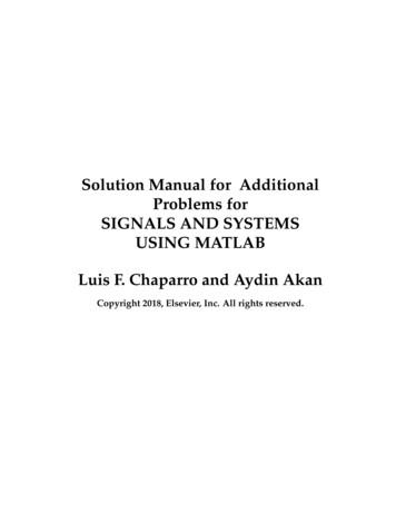
Chaparro-Akan — Signals and Systems using MATLAB0.100.8 Complex functions of time — Consider the complex function x(t) (1 jt)2 for t .(a) Find the real and the imaginary parts of x(t) and carefully plot them with MATLAB. Tryto make MATLAB plot x(t) directly, what do you get? Does MATLAB warn you? Does itmake sense?.(b) Compute the derivative y(t) dx(t)/dt and plot its real and imaginary parts, how dothese relate to the real and the imaginary parts of x(t)?(c) Compute the integralZ1x(t)dt0(d) Would the following statement be true? (remember indicates complex conjugate) Z10Answers:R10 Zx(t)dt 1x (t)dt0x(t)dt 2/3 j1; statement is true.Solution(a)(b) Sincex(t) (1 jt)2 1 j2t j 2 t2 1 t2 j {z}2t {z }imag.realits derivative with respect to t isy(t) dx(t)dRe[x(t)]dIm[x(t)] 2t 2j jdtdtdt% Pr. 0.8clear allt [-5: 0.001:5];x (1 j*t).ˆ2;xr real(x);xi imag(x);figure(7)subplot(211)plot(t,xr); title(’Real part of x(t)’); gridsubplot(212)plot(t,xi); title(’Imaginary part of x(t)’); xlabel(’Time’); grid% Warning when plotting complex signalsfigure(8)disp(’Read warning. MATLAB is being nice with you, this time!’)plot(t,x); title(’COMPLEX Signal x(t)?’); xlabel(’Time’)When plotting the complex function x(t) as function of t, MATLAB ignores the imaginary part.One should not plot complex functions as functions of time as the results are not clear whenusing MATLAB. See Fig. 5 for plots.(c) Using the rectangular expression of x(t) we haveZ01x(t)dt Z01(1 t2 2jt)dt Z01(1 t2 )dt 2jZ01t dt t 2t2t3 j32Copyright 2018, Elsevier, Inc. All rights reserved.10 2 j13

Chaparro-Akan — Signals and Systems using MATLAB0.11(d) The integralZ01 x (t)dt Z012(1 t 2jt)dt Z120(1 t )dt 2jZ1t dt t 0t32t2 j3210 2 j13which is the complex conjugate of the integral calculated in (c). So yes, the expression is true.Real part of x(t)5COMPLEX Signal x(t)?50 50 10 15 5 20 25 5 4 3 2 1012345 10Imaginary part of x(t)10 1550 20 5 10 5 4 3 2 10Time12345 25 5 4 3 2 10Time12345Figure 5: Problem 8: Real and imaginary parts of x(t) (left); complex signal x(t) ignoring imaginarypart.Copyright 2018, Elsevier, Inc. All rights reserved.

Chaparro-Akan — Signals and Systems using MATLAB0.120.9 Hyperbolic sinusoids — In filter design you will be asked to use hyperbolic functions. In thisproblem we relate these functions to sinusoids and obtain a definition of these functions so thatwe can actually plot them.(a) Consider computing the cosine of an imaginary number, i.e., usecos(x) ejx e jx2let x jθ and find cos(x). The resulting function is called the hyperbolic cosine orcos(jθ) cosh(θ)(b) Consider then the computation of the hyperbolic sine sinh(θ), how would you do it? Carefully plot it as a function of θ.(c) Show that the hyperbolic cosine is always positive and bigger than 1 for all values of θ(d) Show that sinh(θ) sinh( θ)(e) Write a MATLAB script to compute and plot these functions between 10 and 10.Answers: sinh(θ) j sin(jθ) and odd.Solution(a) If x jθcos(jθ) 1 θ(e eθ ) cosh(θ)2(b) The hyperbolic sine is defined assinh(θ) 1 θ(e e θ )2which is connected with the circular sine as followssin(jθ) 1 θ(e eθ ) j sinh(θ) sinh(θ) j sin(jθ)2j(c) Since e θ 0 then cosh(θ) cosh( θ) 0, the smallest value is for θ 0 which givescosh(0) 1(d) Indeed,1sinh( θ) (e θ eθ ) sinh(θ)2% Pr. 0.9clear alltheta sym(’theta’);x 0.5*(exp(-theta) exp(theta));y ])gridCopyright 2018, Elsevier, Inc. All rights reserved.

Chaparro-Akan — Signals and Systems using MATLAB0.131/2 exp(θ) 1/2 exp( θ)6000500040003000200010000 10 8 6 4 20θ246810468101/2 exp(θ) 1/2 exp( θ)200010000 1000 2000 10 8 6 4 20θ2Figure 6: Problem 9: cosh(θ) (top) and sinh(θ) (bottom).Copyright 2018, Elsevier, Inc. All rights reserved.

Chaparro-Akan — Signals and Systems using MATLABCopyright 2018, Elsevier, Inc. All rights reserved.0.14

Chapter 1Continuous–time Signals1.1Basic Problems1.1 Consider a finite support signal x(t) t, 0 t 1, and zero elsewhere.(a) Plot x(t 1) and x( t 1). Add these signals to get a new signal y(t). Do it graphically and verifyyour results analytically.(b) How does y(t) compare to the signal Λ(t) (1 t ) for 1 t 1 and zero otherwise? Plot them.Compute the integrals of y(t) and Λ(t) for all values of t and compare them.Answers: x( t 1) is x( t) delayed by 1; y(t) is even, y(0) 2.Solution(a) If x(t) t for 0 t 1, then x(t 1) is x(t) advanced by 1, i.e., shifted to the left by 1 so that x(0) 0occurs at t 1 and x(1) 1 occurs at t 0.x(t 1)x(t)101t1 1x( t)1 10t0x( t 1)1tt012Figure 1.1: Problem 1: Original signal x(t), shifted versions x(t 1), x( t) and x( t 1).1

Chaparro-Akan — Signals and Systems using MATLAB1.2The signal x( t) is the reversal of x(t) and x( t 1) would be x( t) advanced to the right by 1. Indeed,tx( t 1)1x(0)0x(1) 1x(2)The sum y(t) x(t 1) x( t 1) is such that at t 0 it is y(0) 2; y(t) x(t 1) for t 0; andy(t) x( t 1) for t 0. Thus,y(t) x(t 1) t 10 t 1 1 or 1 t 0y(0) 2y(t) x( t 1) t 1or0 t 1 1 or 0 t 1 t 12y(t) t 1 1 t 0t 00 t 1(b) Except for the discontinuity at t 0, y(t) looks like the even triangle signal Λ(t), their integrals arey(t)2 11tFigure 1.2: Problem 1: Triangular signal y(t) with discontinuity at the origin.identical as the discontinuity of y(t) does not add any area.Copyright 2018, Elsevier, Inc. All rights reserved.

Chaparro-Akan — Signals and Systems using MATLAB1.31.2 Given the causal full-wave rectified signal x(t) sin(2πt) u(t)(a) Find the even component of x(t), call it xe (t) and plot it. Is xe (t) periodic? if so, what is its fundamental fundamental period Te ? Would the odd component of x(t) or xo (t) be periodic too?(b) Are xe (t) and xo (t) causal signals? Explain.Answers: xe (t) is periodic, xo (t) is not, both are non-causal.Solution(a) x(t) is called causal because it is zero for t 0, it repeats every 0.5 sec. for t 0.x(t)1xe (t)0.5··· 0.5xo (t) 0.5···0.50.50.50.5···1···1···1 0.5Figure 1.3: Problem 2.(b) Even component xe (t) 0.5[x(t) x( t)] is periodic of fundamental period Te 0.5. The oddcomponent is xo (t) 0.5[x(t) x( t)] is not periodic.(c) xe (t) and xo (t) are non-causal signals as they are different from zero for negative times.Copyright 2018, Elsevier, Inc. All rights reserved.

Chaparro-Akan — Signals and Systems using MATLAB1.41.3 Is it true that (if not true, give correct answer)(a) for any positive integer kZkej2πt dt 0?0(b) for a periodic signal x(t) of fundamental fundamental period T0T0ZZt0 T0x(t)dtx(t)dt t00for any value of t0 ? Consider, for instance, x(t) cos(2πt).(c) cos(2πt)δ(t 1) 1 ?(d) If x(t) cos(t)u(t) then dx(t)/dt sin(t)u(t) δ(t) ?(e) the integralZ e t u(t) δ(t 2)dτ e 2 ? (f) If x(t) cosh(t)u(t) 0.5(et e t )u(t) is dx(t)/dt sinh(t)u(t) δ(t) ?(g) that the power of the causal full-rectified signal x(t) sin(t) u(t) is twice the power of its evencomponent xe (t) 0.5[x(t) x( t)]?Answers: (a) and (b) are true; cos(2πt)δ(t 1) δ(t 1); (g) yes, Pxe 0.5Px .Solution(a) Yes, expressing ej2πt cos(2πt) j sin(2πt), periodic of fundamental period T0 1, then theintegral is the area under the cosine and sine in one or more periods (which is zero) when k 6 0 andinteger. If k 0, the integral is also zero.(b) Yes, whether t0 0 (first equation) or a value different from zero, the two integrals are equal as thearea under a period is the same. In the case x(t) cos(2πt), both integrals are zero.(c) It is not true, cos(2πt)δ(t 1) cos(2π)δ(t 1) δ(t 1).(d) It is true, considering x(t) the product of cos(t) and u(t) its derivative isdx(t)dt d cos(t)du(t)u(t) cos(t)dtdt sin(t)u(t) cos(0)δ(t)(e) Yes,Z e t u(t) δ(t 2)dτ Z 2 eδ(t 2)dτ0 e 2(f) Yes,dx(t)dt 0.5[et u(t) et δ(t)] 0.5[ e t u(t) e t δ(t)] 0.5[et e t ]u(t) δ(t) sinh(t)u(t) δ(t)Copyright 2018, Elsevier, Inc. All rights reserved.

Chaparro-Akan — Signals and Systems using MATLAB1.5(g) The even component xe (t) is a periodic full-wave rectified signal of amplitude 1/2 and fundamentalperiod T1 π.Power of x(t) Z π 1Px 0.5x2 (t)dtπ 0Power of xe (t)Pxe 1πZπ(0.5x(t))2 dt 0.5Px0Copyright 2018, Elsevier, Inc. All rights reserved.

Chaparro-Akan — Signals and Systems using MATLAB1.61.4 The signal x(t) tt 2 t 00 t 2can be written as x(t) t p(t).(a) Carefully plot x(t) and define p(t), then find y(t) dx(t)/dt and carefully plot it.(b) CalculateZty(τ )dτ and comment on how your result relates to x(t).(c) Is it true thatZ 2Zx(τ )dτ ?x(τ )dτ 2 0Answers: y(t) 2δ(t 2) u(t 2) 2u(t) u(t 2) 2δ(t 2); yes, it is true.Solution(a) See Fig. 4ax(t) t [u(t 2) u(t 2)] Derivative {z}p(t)x(t)2 2t2y(t)1(2)t2 2 1( 2)Figure 1.4: Problem 4y(t) dx(t) 2δ(t 2) u(t 2) 2u(t) u(t 2) 2δ(t 2)dt(b) IntegralZt00y(t )dt 0 tt 0t 2 2 t 00 t 2t 2which equals x(t).(c) Yes, because x(t) is an even function of t.Copyright 2018, Elsevier, Inc. All rights reserved.

Chaparro-Akan — Signals and Systems using MATLAB1.21.7Problems using MATLAB1.5 Sampling signal and impulse signal — Consider the sampling signalδT (t) Xδ(t kT )k 0which we will use in the sampling of analog signals later on.(a) Plot δT (t). FindZtδT (τ )dτssT (t) and carefully plot it for all t. What does the resulting signal ss(t) look like? This signal has beencalled the “stairway to the stars.” Explain.(b) Use MATLAB function stairs to plot ssT (t) for T 0.1. Determine what signal would be the limit asT 0.(c) A sampled signal is Xxs (t) x(t)δT (t) x(kTs )δ(t kTs )k 0Let x(t) cos(2πt)u(t) and Ts 0.1. Find the integralZ txs (t)dt and use MATLAB to plot it for 0 t 10. In a simple way this problem illustrates the operation of adiscrete to analog converter which converts a discrete-time into a continuous-time signal (its cousinis the digital to analog converter or DAC).RtPPAnswers: (a) ss(t) k x(kTs )u(t kTs ).k 0 u(t kT ); (c) xs (t)dt Solution(a) The sampling signal is a sequence of unit impulses at uniform times kT , for t 0. The integralZ t X Z t XXssT (t) δ(t kT )dt u(t kT )δ(t kT )dt k 0k 0 k 0This signal is called the “stairway to the stars” (ssT (t)) for obvious reasons.(b)(c) The following script will display the signal ss(t) and the conversion to analog (just uncomment thedesired signal and comment the not desired signal).% Pr. 1 5 parts (b) and (c)clear all; clfT 0.1; t 0:T:10;%f t; % part (b)f cos(2*pi*t); % part (c)figure(6)stairs(t,f);grid%axis([0 10 0 10]) % part (b)axis([0 10 -1.1 1.1]) % part (c)hold onplot(t,f,’r’)hold offWhen f (t) t 1 the output looks like a digitized line with unit slope and cut at 1 (see figurebelow), similarly when f (t) cos(2πt) the output looks like a digitized sinusoid.Copyright 2018, Elsevier, Inc. All rights reserved.

Chaparro-Akan — Signals and Systems using MATLAB1.810190.880.670.460.2504 0.2 0.43 0.62 0.81 10012345678910012345678910Figure 1.5: Problem 5: ‘Digitized’ ramp and cosine signals using ’stairway to stars’Copyright 2018, Elsevier, Inc. All rights reserved.

Chapter 2Continuous–time Systems2.1Basic Problems2.1 The input-output relationship of a system isy(t) sign(x(t)) (1 1if x(t) 0if x(t) 0where x(t) is the input and y(t) the output.(a) Let the input be x(t) sin(2πt)u(t), plot the corresponding output y(t). What is theoutput of the system if we double the input? That is, what is the output y1 (t) if the inputx1 (t) 2x(t) 2 sin(2πt)u(t)? Is the system linear or not?(b) Is the given system time-invariant?Answers: output y(t) SolutionP k 0p(t k) with p(t) u(t) 2u(t 0.5) u(t 1).(a) x(t) sin(2πt)u(t) is zero for t 0 and repeats periodically every T0 1. Thus,y(t) Xk 0p(t k), p(t) u(t) 2u(t 0.5) u(t 1)If the input is 2x(t) the output is the same as before, so the system is non-linear.(b) The system is time-invariant: if input x(t τ ) the output is y(t τ ) for any value of τ .1

Chaparro-Akan — Signals and Systems using MATLAB2.22.2 Consider the following problems about the properties of systems.(a) A system is represented by the ordinary differential equation dz(t)/dt w(t) w(t 1)where w(t) is the input and z(t) the output.i. How is this system related to an averager having an input/output equationZ tz(t) w(τ )dτ 2 ?t 1ii. Is the system represented by the given ordinary differential equation LTI?(b) If we consider the current i(t) the input of a capacitor, with a zero initial voltage across it,the voltage across the capacitor –or the output— is given byZ ti(τ )dτvC (t) 0i. Is this capacitor time-invariant? If not, what conditions would you impose to make ittime-invariant?ii. If we let i(t) u(t) what is the corresponding voltage vC (t)? If we delay the currentsource so that the input is i(t 1), find the corresponding voltage across the capacitorand indicate if this result shows the capacitor is time invariant.(c) An amplitude modulation system has an input/output equation t y(t) x(t) sin(2πt)i. Let x(t) u(t), plot the corresponding output y(t) sin(2πt)u(t)ii. If the input is delayed, i.e., the input is x1 (t) x(t 0.5) u(t 0.5), plot thecorresponding output y1 (t) x1 (t) sin(2πt), and use this result to determine whetherthe given AM system is time-invariant.Answer: (a) z(t) solution of differential equation with initial condition of 2; (b) If i(t) 0 fort 0, system is TI; (c) If x(t 0.5) u(t 0.5) the output is y1 (t) sin(2πt)u(t 0.5).Solution(a) Derivativedz(t) w(t) w(t 1)dtwhich excludes the initial condition of 2. System is LTI if initial condition is zero.(b)i. If input is i(t µ) then the output is letting η τ µZ tZ 0Z t µi(τ µ)dτ i(η)dη i(η)dη vc (t µ)0 µ0that is, provided that i(t) 0 for t 0, the system is time-invariant.Copyright 2018, Elsevier, Inc. All rights reserved.

Chaparro-Akan — Signals and Systems using MATLABii. If i(t) u(t) then vc (t) Rt02.3u(τ )dτ r(t). If we shift the inputs i1 (t) i(t 1) u(t 1) the previous output is shifted, so system is time-invariant.(c) If x(t) u(t) then y(t) sin(2πt)u(t) while corresponding to x(t 0.5) u(t 0.5) isy1 (t) sin(2πt)u(t 0.5) indicating the system is not time-invariant as y1 (t) is not y(t 0.5).sin(2 π t) heaviside(t) 0.500.5theaviside(t 1/2) sin(2 π t)11.5 0.500.5t11.5Figure 2.1: Problem 2(c)Copyright 2018, Elsevier, Inc. All rights reserved.

Chaparro-Akan — Signals and Systems using MATLAB2.42.3 The following problems relate to linearity, time–invariance and causality of systems.(a) A system is represented by the equation z(t) v(t)f (t) B where v(t) is the input, z(t)the output, f (t) a function and B a constant.i. Let f (t) A, a constant. Is the system linear if B 6 0? linear if B 0? Explain.ii. Let f (t) cos(Ω0 t) and B 0 is this system linear? time-invariant?iii. Let f (t) u(t) u(t 1), the input v(t) u(t) u(t 1), B 0, find the correspondingoutput z(t). Let then the input be delayed by 2, i.e., the input is u(t 2) u(t 3) andf (t) and B be the same, determine the corresponding output. Using these results, isthe system time invariant?(b) An averager is defined asy(t) 1TZtx(τ )dτt Twhere T 0 is the averaging interval, x(t) and y(t) are the system input and output.i. Determine if the averager is a linear system.ii. Let T 1, x(t) u(t), calculate and plot the corresponding output, delay then theinput to get x(t 2) u(t 2), and calculate and plot the corresponding output.From this example, does the system seem time invariant? Explain. Can you show itin general.iii. Is this system causal? Give an example to verify your assertion.Answer: (a) If f (t) v(t) u(t) u(t 1) then z(t) u(t) u(t 1), and if input isv1 (t) u(t 2) u(t 3) output is z1 (t) v1 (t)f (t) 0; (b) If x(t) u(t) then y(t) r(t) r(t 1)and if x1 (t) u(t 2) the corresponding output is y1 (t) y(t 2).Solution(a)i. z(t) Av(t) B, system is linear if B 0, non-linear otherwise.ii. z(t) v(t) cos(Ω0 t) is linear but time-varying.iii. If f (t) v(t) u(t) u(t 1), B 0 then z(t) u(t) u(t 1), and if we shift v(t)so the input is v1 (t) u(t 2) u(t 3) the output is z1 (t) v1 (t)f (t) 0 which isdifferent from z(t 2), so the system is time-varying.(b)i. The system is linear:1TZtA[Ax1 (τ ) Bx2 (τ )]dτ Tt TZtt TBx1 (τ )dτ TZtx2 (τ )dτ Ay1 (t) By2 (t)t Twhere yi (t), i 1, 2, are the

discrete-time signals (use the stem function). Superimpose the analog and the discrete-time signals for 0 t 3; use subplot to plot the four figures as one figure. You also need to figure out how to label the different axes and how to have the same scales and units. Answers: For T s 1 the discre