Transcription
Laser remote sensing of epipelagic fishesJames H. ChurnsideNOAA Environmental Technology Laboratory325 BroadwayBoulder, CO 80303John R. HunterNOAA Southwest Fisheries Science CenterP.O. Box 271La Jolla, CA 92038ABSTRACTAirborne lidar is being considered as a tool for fish detection and for fisheries surveys. Detectionhas been demonstrated, and an imaging lidar has been developed to detect and identify fish for commercialfisheries. For survey work, a simpler radiometric lidar is being investigated, and preliminary results suggestthat such a lidar can be very useful for biomass estimation.Keywords: lidar, fisheries, ocean optics1. INTRODUCTIONAirborne remote sensing of fish is not new. Sea birds are very capable of locating fish near thesurface of the ocean. Using a similar technique, spotter pilots are used by fishing fleets to locate fish anddirect the boats to the fish.1,2 During the day, fish schools can be directly observed near the surface. Atnight, the bioluminescence stimulated by the movement of fish is observed. From visual observations, thesepilots are able to identify species and to make estimates of school size. These observations are also usedby fisheries managers in some cases. For California waters, pilot reports have been collected each year for30 years to provide a time series of the relative abundance of anchovy, mackerel, and sardine.1 In the lastfew years, these data have been used as an index of fish abundance in annual stock assessments.3These airborne data have been valuable to fishery managers because of difficulties with moretraditional survey techniques. Traditional direct surveys include ichthyoplankton sampling, trawling, andacoustic surveying. These are limited in coverage area by the speed and cost of surface ships. In addition,many schooling fishes may avoid surface vessels,4 biasing survey results.Despite their usefulness, visual observations have several difficulties. The first is that they areseverely depth limited. The detection depth limit is about one diffuse attenuation length, although thisdepends strongly on illumination, sea state, and the skill of the individual observer. Photographic recordshave been used in an attempt to eliminate observer-to-observer differences.5,6 These are still subject toillumination and sea state problems.
For these reasons, laser systems are being developed for application in fisheries. Laser illuminationwill allow penetration to greater depths than passive observations, and range gating will mitigate difficultiescaused by the rough air-sea interface.An airborne fish-lidar also has important commercial fishing applications. In many parts of theworld, tuna fisheries (yellowfin and skipjack tuna), and small pelagic fisheries (sardine, anchovy, mackerel,menhaden) employ airplanes or helicopters to locate fish schools for the industry. Substitution of visualobservations by a lidar would greatly increase the effectiveness of aerial observations, thereby increasingindustry efficiency. In addition, improved aerial fish finding may solve a critical fishery bicatch problemin the yellowfin tuna fishery of the Eastern Tropical Pacific (ETP). In the ETP, tuna are captured by locatingdolphin herds, and this methods often produces adverse results, including dolphin mortality. An airbornesensor that could detect and track schools of larger tunas unassociated with dolphins would offer anecologically sound alternative to the current method.A rather generic block diagram of a fish lidar is presented in Fig. 1. The laser generates a pulse oflight in the blue-green region of the visible spectrum, where the absorption of sea water is minimized. Thelaser beam is appropriately shaped with optics, represented by a small lens in the figure, and directed througha scanning system. Laser light reflected by fish and by small particles in the ocean is directed into atelescope by the same scanning system, and detected by an optical detector located either at the focal planeor the image plane of the telescope. The resulting electronic signal is sent to a computer after suitableelectronic conditioning and digitization.Three types of lidar systems are possible forapplication in fisheries, each providing a differentview of fish schools. The simplest, radiometric lidar,has no scanning system, and the detector is a singleelement detector. Each pulse provides a full depthprofile of the lidar return at a fixed direction from theaircraft, usually just off nadir. As the aircraft movesalong, the system provides a two-dimensional pictureof fish schools, where one axis is depth and the otheris the target strength integrated over the width ofswath cut by the lidar. The second type, imaginglidar, produces a horizonal image at a fixed depthwithout scanning. A gated imaging detector is used,and each pulse provides a horizontal image at a depthdetermined by the setting of the range gate; theseimages of individual pulses are patched together asFig. 1. Block diagram of a fish lidar system.the airplane moves to produce a composite image.The third type, volumetric lidar, uses a scanningsystem and a single-element detector. Each pulse provides a single profile with depth, but the scanningsystem is used to construct a volume, or three-dimensional image, from the individual pulses.Volumetric lidars have been used for bathymetric applications, as described in other chapters of thisvolume, and fish have been observed during bathymetric operations. Imaging lidars have been evaluated
for fish finding, and a commercial unit (Fisheye ) is being marketed by Kaman Aerospace. A number ofradiometric systems have also been used for fish detection.2. LIDAR OBSERVATIONSIn 1981, Squire and Krumboltz7were among the first to document lidardetection of fish schools. Their systemwas a Navy radiometric lidar (ORIC)mounted on a helicopter and flown offNew Jersey. Reported lidar parameters areprovided in Table 1. Fig. 2 is a plot of thevertical cross section of a school inferredfrom the lidar data. Each numberedsection corresponds to a lidar pulse.Fig. 2. Vertical cross section of an unidentified fishschool from the ORIC lidar (Ref. 7).Table 1. Parameters of several existing fish lidar systems.System NameORICMakrel-2Osprey FLOEFishEye agingWavelength532 nm532 nm532 nm532 nm532 mPulse Length15 nsec15 nsec15 nsec10 nsecPulse Energy70 mJ35 mJ100 mJ170 mJPulse RepetitionRate15 Hz20 Hz1-20 Hz10-30 Hz30 HzLaser Divergence48 mrad1 mrad2 mrad50 mrad160 mrad15 cm20 cm20 cmReceiver ApertureDiameterReceiver Fieldof View48 mradElectronicBandwidth2-13 mrad40 MHZ25 mrad100 MHZ100 MHZShutter SpeedAmplifierSample Rate160 mrad20-120 nseclinearlinearlogarithmiclogarithmiclinear40 MHZ250 MHZ1 GHz30 Hz
Since 1982, the Institute ofAtmospheric Optics in Russia has usedairborne radiometric lidar to detect fish in thesea. The parameters of their most recentconfiguration, referred to as the Makrel-2,8,9are also presented in Table 1. This systemtransmits linear polarization and receivesboth the co-polarized and the cross-polarizedreturn, providing additional informationabout scattering targets. Fig. 3 is a samplereturn from the Makrel-2 showing a clearwater return (a) and a return including a fishschool at a depth of about 11 m (b). Theclear water return shows an intensity (curve1) that decreases with depth and adepolarization ratio (curve 2) that increaseswith depth. The fish school can be identifiedby an increase in the received intensity and adecrease in the depolarization ratio at 11 m.Development of the Osprey lidar10by Remote Sensing Industries began in 1990.This device is a radiometric lidar designed todetect tuna from a helicopter.Theparameters of this lidar are also presented inTable 1. The most extensive test of thissystem occured between September 25 toOctober 20, 1992, when it was installed onthe helicopter of the CMS purse seinerCaptain Vincent Gann, and operated on adaily basis for a total of approximately 160hours in the eastern tropical Pacific. Fig. 4 isan example of data obtained during this test.The single-profile display on the left clearlyshows a fish return at a depth of 50 feet. Thiswas confirmed to be a school of tuna; thecommercial purse seiner harvested thisparticular school. It contained 2.5 tons of 3-5kg skipjack and yellowfin tuna, 0.5 tons ofbigeye tuna over 2 kg, 31.5 tons of skipjackand yellowfin tuna under 3 kg, 3.2 tons ofbigeye tuna under 2 kg, and 0.3 tons of smallblack skipjack tuna, or a total of 38 tons oftuna. This was one of the larger schoolscaught on what was not a very successfulFig. 3. Depth record of a lidar pulse containing fishat 11 m from the Makrel-2 lidar (Ref. 9). IntensityIlin of the return (curve 1) is on the left vertical axis,and depolarization ratio Q (curve 2) is on the right.Fig. 4. Depth profile and time/range imagecontaining a tuna school at pulse 285 from theOsprey lidar (Ref. 10).
cruise.The National Oceanic andAtmospheric Administration (NOAA)Experimental Oceanic Fish Lidar (FLOE),also a radiometric lidar, is being developedfor aerial surveys of epipelagic fishes.Although it is capable of flying in a smallaircraft, it has been operated on the researchtrawler R/T David Starr Jordan, which isalso equipped with sonar and acoustic echosounders. The pertinent parameters arepresented in Table 1. Normally, this lidartransmits parallel polarization and receivesperpendicular polarization. This seems toprovide the best contrast between fish andvolumetric scattering in the water column.Fig. 5 is a typical fish-school image from theSeptember 1995 cruise. The top portion ofthe image is the raw, logarithmic amplifieroutput. The bottom portion of the image hasbeen processed to separate the fish returnfrom the water return. This processing is notnecessary for fish detection, since theenhancement of the signal corresponding tofish is clear in the unprocessed image.However, for quantitative analysis of themagnitude of the fish return, that returnneeds to be isolated.Fig. 5. Time/range image of a fish school from theFLOE lidar. Upper image is the unprocessedimage, and the lower image has been processed toseparate the fish reflection from the backgroundwater reflection.In the simplest case, we assume that the water properties are constant with depth, so that the returnfrom water only can be expressed as(1)where S is the linear lidar signal, z is depth, a is a signal amplitude that depends on parameters such as laserenergy and pulse width, water backscatter coefficient, receiver aperture, detector responsivity, etc., " is theattenuation coefficient of the laser in the water, h is the height of the lidar above the surface, n is the indexof refraction of the water, and b is the contribution of background light to the signal. If fish are present atsome depth, there is an additional contribution to the signal at that depth that depends on the backscattercoefficient of the fish, so
(2)where f and w are the backscatter coefficients of the fish and of the water. This model also assumes thatthe attenuation of light by the fish can be neglected.The processing steps used to obtain the separated image in Fig. 5 follow from these two equations.First, a, ", and b are estimated by choosing three depths on each return that are free of fish and solving theresulting three equations. These three parameters are used with Eq. (1) to obtain an estimate of the waterreturn, Sw. The logarithm of this is subtracted from the logarithm of the measured signal to get(3)Exponentiating this quantity and subtracting 1 provides the fish backscatter coefficient normalized by thewater backscatter coefficient. This quantity is proportional to the number of fish within the depth-resolutionelement.Fig. 6 is the echo sounder record ofthe same fish school. Since the twoinstruments areseparated by about 20 m on the ship, the twoimages of the fish school would not beexpected to be identical. It is clear,however, that the general features of schooldepth, thickness, and fish density are verysimilar in the two images.A scanning lidar, the LARSEN 500,Fig. 6. Echo sounder time/range image of the samewas used to collect data during the 1995school as in Fig. 5.herring fishery off of the east coast ofVancouver Island in Canada.11 This lidar is not included in Table 1. A sophisticated signal-processingtechnique was developed to locate fish schools precisely, despite low signal levels.The FishEye lidar is an imaging system designed primarily for fish detection. It images the outlineof large fish or mammals or the outline of schools. The resolution depends on water clarity, but a few tensof cm is typical. This resolution provides information that can help in species identification, but gives littleinformation on depth. This is disadvantageous for biomass estimation of schooling fish since schoolthickness is needed for the computation of the biomass of a school. The system is designed so that the gatemust be set for a particular depth, and all one can tell is whether the target is above or below that depth.
Targets above the gated depth will appear as a shadow against the water return, those below will appearbrighter than the surroundings. This system was extensively tested off the coast of Chile during a three-weekperiod in July 1995. Fig. 7 is a reflection-mode image of a school of fish in the net around a fishing boat.The shadow of the boat is clearly visible on the right of the image. The range gate for this image, and hencethe fish school, is from 12 to 26 m. Fig. 8 is a shadow-mode image of another school. The depth gate is thesame, so these fish are in the upper 12 m of the ocean.Fig. 7. Reflection image of a school of anchovies Fig. 8. Shadow image of a school of anchovies offChile from the FishEye lidar (provided by Kamanin a net around a fishing boat off Chile from theFishEye lidar (provided by Kaman Aerospace). Aerospace).3. MODELING EFFORTSMany of the modeling issues relevant to fisheries lidar are the same as those for other lidar systems.However, in this case, the optical characteristics of the fish also need to be determined. In 1974, Murphree,et al12 concluded, "The results from the developed mathematical model, using input parameters of presentlyavailable equipment and estimates of fish school density and reflectivity, reveal that the power received atan airborne detector from fish reflected incident laser radiation and the S/N are of sufficient magnitude tolocate fish schools with an airborne remote laser sensing system." The estimates of fish school density andreflectivity used in this study were that 50% of the cross-sectional area of the beam intercepted fish, and thatthe reflectivity of those fish was 5%. Depths of up to 14 m were considered.A more recent study13 used a Monte-Carlo calculation, and also concluded that fish detection waspossible. This study considered a layer of fish 5 m thick at a depth of 5 m. This study used a fish reflectivityof 5%, based on Reference 12. Two fish densities were used in this study, 50 m-3 and 25 m -3, with anassumed fish cross section of 20 cm2. For a 5-m thick layer, the product of the number density, the crosssectional area of each fish, and the layer thickness results in roughly 50% and 25% coverage of the layer bythe beam, so that fish density is also similar to that used in Reference 12. Fig. 9 is a plot of depth profilesof the intensity of a lidar return using that model and reproduced from Reference 9.For many purposes, a much simpler model can be used. A commercial spreadsheet program is ideal
for varying the parameters of a lidar system, the water, or the fish, and observing the consequences. Thisrequires that the physics of the model be simplified. The full effects of multiple scattering are particularlydifficult to incorporate into a spreadsheet model that will perform the calculations in a reasonable time.However, in many cases, such effects can be parameterized by, for example, an increased beam divergence.If the initial beam divergence is larger that the beam spreading, even this is not needed. Fig. 10 is a plot ofthe signal return from a school of fish at a depth of 5 m calculated using such a spreadsheet. In this case,a measured profile of the diffuse attenuation coefficient in the Southern California Bight was used tocalculate the return from a system with a fairly wide field of view.Fig. 9. Monte-Carlo calculations of the depthprofiles of lidar returns from a layer of fish at adepth of 5 m (Ref. 9). Fields of view of 2 mrad(curve 1), 4 mrad (curve 2), and 8 mrad (curve 3)were used.Fig. 10. Commercial spreadsheet calculation of thedepth profile of a lidar return from a layer of fish ata depth of 5 m.3. FISH SCHOOL CHARACTERISTICSPerformance of fish lidar, particularly for fishery management, depends upon the three biologicalparameters discussed below: fish reflectivity, school packing density, and depth. Fish reflectivity is of keyimportance not only because it is needed for forecasting maximum fish-detection depth, but, mostimportantly, because it forms a direct computational link between the strength of the lidar signal and thenumber of fish or biomass. Squire and Krumboltz7 assumed a reflectivity of 50% in order to estimate thearea of the fish intercepted by their lidar. Krekova, et.al.13 followed Murphree, et.al.12 in assuming areflectivity of 5%. Fredriksson et.al.14 measured the lidar return from fish, but their system was notcalibrated. Benigno and Kemmerer15 measured the reflectivity of menhaden in the sea using natural lightand got a value of less than 1% across the blue-green portion of the spectrum. Churnside and McGillivary16made calibrated measurements on dead fish, and obtained reflectivities of 18-26% for blue light and 15-22%for green light, depending on species. Clearly, more work on fish reflectivity is needed.A direct measure or index of packing density of fish within a school is also essential if schoolbiomass is to be accurately estimated. Packing density of schools is highly variable because it is a functionof feeding, fright, swimming behavior, diel rhythms, and other factors. Procedures used to measure packing
density in the sea, such as dropping cameras through schools, counting the fish in purse-seine catches, anddriving ships equipped with echo sounders over schools, generally frighten the fish and increase density.The most striking difference is between night and day schools. Night schools are often so diffuse that someresearchers have concluded that schooling ceases, although purse-seine fisheries for sardine, anchovy, andmenhaden use bioluminescence to detect and catch schools at night.Clearly, fish size affects packing density, and attempts have been made to express an average packingdensity in terms of fish length, L.17,18 Based on laboratory observations, densities of L-3 and (2.44L)-3 havebeen suggested (by Refs. 17 and 18, respectively). However, average packing densities in the open oceanare typically much lower than in laboratories. A summary of open-ocean data for sprat, herring, and saithesuggests that the packing density for these fish is lower than either of the laboratory-based models.19 Thatis, the nearest neighbor distance is generally less that 2.44L.Measurements made from underwater photographs demonstrate a large range of packing densityunder natural conditions. For Northern anchovy during the day, a range of nearest-neighbor distances from0.79L to 1.63L was measured.20 This corresponds to packing densities of 50 to 366 fish per cubic meter.For Japanese anchovy at night, nearest-neighbor distances varied from 7.8L to 12L, corresponding to apacking-density range of 0.25 to 0.87 m-3.21 Jack mackerel, measured at night, had nearest-neighbordistances of 18L to 21.5L and packing densities of 6.6 to 19.5 m-3.22 Packing density will even vary greatlywithin a school. One school of herring was found to have densities from fewer than 0.1 m-3 to more than8 m-3.19 Observations of sardine schools suggest that the leading edge of a crescent-shaped sardine schoolhas a much higher density than the trailing edge.23School packing density also seems to vary greatly between day and night. The average density ofthe South African pilchard was found to be 4.3 times as great in the day as at night.30 The typical densityof adult anchovy schools was estimated to be 20 times that at night.24 School thickness does not appear tovary greatly between day and night.25The next parameter to consider is school depth. For most species, some fish will be found at depthsthat exceed even the most optimistic forecasts for airborne lidar performance, especially during the day. Onepossible exception may be the Pacific soury, a commercial species that is limited in range to the upper fewmeters of the water column.One common feature of the vertical distribution of epipelagic schooling fishes is that the schools arecloser to the surface at night. This has been documented by acoustic records off daily migration of fish fromgreater depths to the surface at night26 and by surface observations.27 The swimming patterns of yellowfintuna tracked with acoustic transmitters28 show depth changes of 100 m several times in an hour. These dataalso show that the daytime vertical range was between 50 and 150 m, while the nighttime range was between0 and 100 m in depth.The diurnal difference in depths seems to be related to the amount of light required for the fish tosee each other. Whitney29 reviewed data on visual thresholds for schooling and concluded that sufficientlight existed in the sea for schooling to continue at night if the fish were close enough to the surface. Thisimplies that the nighttime depth of schooling is a function of ambient light, water clarity, and species. Fig.11 is a plot of the visual threshold for schooling as a function of chlorophyll concentration for northern
Note that as the chlorophyllanchovy. 30concentration increases, the maximum depthpenetration of a lidar is expected to decrease. Underthese conditions, the fish will come closer to thesurface where they can more easily be detected.Even during the day, sardines appear to stayrelatively close to the surface. Three echo-soundersurveys of sardine depth distributions off Japan31found 99.1%, 93.2%, and 92.9% of the fish in theupper 26 m of the ocean. Anchovy range somewhatdeeper. Three daytime acoustic surveys of anchoviesoff California4 found 75%, 65%, and 70% of the fishwithin the upper 50 m. Depth distributions of thelarvae of four species in the Southern CaliforniaBight have been approximated by the Weibulldistribution:(4)Fig. 11. Estimates of the maximum depth ofnorthern anchovy schools at night from Ref.27 for two illumination conditions andvarying chlorophyll concentrations. Darklyshaded area indicates where no schooling isexpected; lightly shaded area indicates depthrange of schooling threshold, with thegeometric mean indicated by the dotted line.where k is the biomass per unit area in the upper zmeters, K is the total biomass per unit area, z0 is themean depth, and J is a shape parameter (unity for theexponential distribution). The parameters for thefour species are listed in Table 2.One of the most variable aspects of fishschools is size. No evidence exists that schoolsconcentrate around a certain optimum size. In some boreal coastal pelagic fishes, such as herring, saithe,Table 2. Fitted parameters of the Weibull distribution for depth distribution of four species of fish inthe Southern California Bight.SpeciesK c Mackerel0.0002651Sardine0.13101
and sprat, school sizes vary by a factor of 10,000 or more.19 Similarly, the areas of daytime anchovy schoolsrange from less than 5 m2 to more than 50,000 m2. Small schools are by far the most numerous, but mostof the biomass of a stock may be concentrated in relatively rare, very large schools. For example,cumulative frequency distributions of the horizontal areas of schools indicate that 50% of anchovy schoolsare less than 30 m in diameter, and 90% of the total area of all schools was produced by schools larger than30 m.32 Another study24 reported that most anchovy schools were 5-30 m in diameter and 4-15 m thick.While these smaller schools were common all year, larger schools, with 25-30 m diameters and 12-40 mthick, appeared in fall and winter.While the size of a school is often described in terms of a diameter, schools are not always circular.They can be described as ovoid, ameboid, ribbon like, and crescent shaped. The advancing edge of crescentshaped schools is often convex.23 Nighttime anchovy schools tend to be more elongated that daytimeschools.27 Accelerated swimming can cause ovoid schools to become more elongated.33 Epipelagic fishschools also tend to be larger in horizontal extent than in thickness. Echo sounder measurements of sardineschools provided a mean school thickness that varied between 3.4 m and 3.9 m for different surveys, withnearly all schools less than 10 m thick.34,35 The median thickness of anchovy schools appears to be about4 m, but values range up to 19 m.4 One estimate of school shape from older data suggests that alength:width:thickness relationship of 3:2:1 is not uncommon.17 More recent measurements of the meanratio of the "crosswise" horizontal dimension to thickness for nine surveys of herring, saithe, and spratobtained values of 1.7 to 4.7, with a median ratio of 2.6.19 This report pointed out that schools tend tobecome thinner when they get close to either the surface or the bottom, and tend to be more spherical in openwater; schools within a few meters of the surface had length-to-thickness ratios as large as ten. Anchovyschools also are very thin at night, when they are close to the surface.27An additional factor to consider is that schools of pelagic fishes are often arranged in distinctaggregations called shoal groups or school groups.5,36,37 These groups have definite coherence, such that thepresence of one group will decrease the probability of another group within 13-17 km. These groups willmove considerable distances as a unit. This patchiness affects the design of an aerial survey or search.3. SURVEY DESIGN CONSIDERATIONSAn optimal survey minimizes potential biases, while delivering the greatest statistical precisionwithin cost constraints. A fundamental assumption of resource surveys is that the surveyed area enclosesall or nearly all of the stock under consideration. This assumption is violated frequently because surveyboundaries are set by costs rather than habitat boundaries. Visual or passive-imaging aerial surveys canminimize the survey area bias in the horizontal dimensions because of their low cost per survey mile, butthey produce a large bias in the vertical dimension because of the limited depth penetration. Airborne lidarsurveys can also minimize the horizontal area bias, and greatly reduce the vertical or volume bias fordaylight surveys. At night, it is possible that most pelagic species (mackerel, anchovy, sardines, menhaden,and possibly tuna) may be fully recruited into a lidar survey volume.For some time to come, accurate fish identification in aerial surveys may remain restricted to about1 attenuation length and the identity of lidar targets detected below that depth will depend on localknowledge and voucher specimens. Similarly, acoustic surveys usually include trawling for approximateidentification of acoustic targets and specimens for determining age composition and growth. In
ichthyoplankton surveys (fish eggs and larvae), on the other hand, species are identified absolutely. If anestimate of absolute biomass is the needed, the ideal approach may be to combine lidar surveys with acousticand/or ichthyoplankton surveys. Acoustic and airborne lidar surveys are quite complementary. Echosounders mounted on ship hulls cannot be used for targets in the upper 5-10 meters of the ocean, and sidelooking sonars are also not effective in same region because of surface and wave inference. The depth rangeof target overlap between lidar and acoustic methods, about 10-40 meters, allows intercalibration betweenacoustics and lidar. Another interesting contrast is that acoustics are most effective during the day whenschools are deeper, while night may be the preferred time for lidar because schools may be fully recruitedinto the surveyed volume. Nighttime lidar surveys are also less effected by background light. Both methodsneed trawling to confirm species identification .There is also merit in combining airborne lidar surveys with ichthyoplankton surveys. Because fewerassumptions are required, ichthyoplankton methods, particularly daily egg production (DEP) and relatedmethods,37 are potentially the most accurate for estimating biomass of epipelagic fishes but they are also themost costly. Vessel progress is slow because of frequent stops to take plankton tows (a tow every 4 nauticalmiles is recommended), and the vessel must also be used for trawling, since specimens are needed toestimate the weight-specific production of eggs. Airborne lidar and DEP methods might profit greatly frombeing combined. The slow DEP method could be greatly enhanced by a rapid method for discovering spatialboundaries, while the absolute abundance estimates provided by the DEPM may be best way to covertschool targets into biomass. In addition, the sampling effort on board the vessel could be allocated on thebasis of the abundance of lidar detected fish schools. Such an adaptive sampling strategy would greatlyimprove the precision of the biomass estimate. Similar arguments were advanced by Shelton et.al.38 whodeveloped methods for combining DEP surveys with acoustics and trawls. These authors stressed the valueof combining absolute abundance estimates of relatively low precision, provided by their DEP estimate,with the relatively precise measurement of relative abundance provided by ac
Airborne remote sensing of fish is not new. Sea birds are very capable of locating fish near the surface of the ocean. Using a similar technique, spotter pilots are used by fishing fleets to locate fi