WIXLIB

Learning Hatching for Pen-and-Ink Illustration of Surfacestransfer spatially-varying textures from source to target geometryusing nonparametric synthesis. Jodoin et al. [2002] model relativelocations of strokes, but not conditioned on a target image or object.Kim et al. [2009] employ texture similarity metrics to transferstipple features between images. In contrast to the precedingtechniques, our method maps to hatching properties, such asdesired tone. Hence, although our method models a narrower rangeof artistic styles, it can model these styles much more accurately.A few 2D methods have also been proposed for transferring stylesof individual curves [Freeman et al. 2003; Hertzmann et al. 2002;Kalnins et al. 2002] or stroke patterns [Barla et al. 2006], problemswhich are complementary to ours; such methods could be useful forthe rendering step of our method.A few previous methods use maching learning techniques to extract feature curves, such as contours and silhouettes. Lum and Ma[2005] use neural networks and Support Vector Machines to identify which subset of feature curves match a user sketch on a givendrawing. Cole et al. [2008] fit regression models of feature curvelocations to a large training set of hand-drawn images. These methods focus on learning locations of feature curves, whereas we focuson hatching. Hatching exhibits substantially greater complexity andrandomness than feature curves, since hatches form a network ofoverlapping curves of varying orientation, thickness, density, andcross-hatching level. Hatching also exhibits significant variation inartistic style.3.OVERVIEWOur approach has two main phases. First, we analyze a hand-drawnpen-and-ink illustration of a 3D object, and learn a model of theartist’s style that maps from input features of the 3D object to targethatching properties. This model can then be applied to synthesizerenderings of new views and new 3D objects. Shortly we present anoverview of the output hatching properties and input features. Thenwe summarize the steps of our method.Hatching properties. Our goal is to model the way artists drawhatching strokes in line drawings of 3D objects. The actual placements of individual strokes exhibit much variation and apparent randomness, and so attempting to accurately predict individual strokeswould be very difficult. However, we observe that the individualstrokes themselves are less important than the overall appearancethat they create together. Indeed, art instruction texts often focus onachieving particular qualities such as tone or shading (e.g., Guptill[1997]). Hence, similar to previous work [Winkenbach and Salesin1994; Hertzmann and Zorin 2000], we model the rendering processin terms of a set of intermediate hatching properties related to toneand orientation. Each pixel containing a stroke in a given illustrationis labeled with the following properties.—Hatching level (h {0, 1, 2}) indicates whether a region containsno hatching, single hatching, or cross-hatching.—Orientation (φ1 [0 . . . π ]) is the stroke direction in image space,with 180-degree symmetry.—Cross-hatching orientation (φ2 [0.π ]) is the cross-hatch direction, when present. Hatches and cross-hatches are not constrainedto be perpendicular.—Thickness (t ) is the stroke width.—Intensity (I [0.1]) is how light or dark the stroke is.—Spacing (d ) is the distance between parallel strokes.—Length (l ) is the length of the stroke. 1:3The decomposition of an illustration into hatching properties isillustrated in Figure 2 (top). In the analysis process, these propertiesare estimated from hand-drawn images, and models are learned.During synthesis, the learned model generates these properties astargets for stroke synthesis.Modeling artists’ orientation fields presents special challenges.Previous work has used local geometric rules for determining strokeorientations, such as curvature [Hertzmann and Zorin 2000] or gradient of shading intensity [Singh and Schaefer 2010]. We find that,in many hand-drawn illustrations, no local geometric rule can explain all stroke orientations. For example, in Figure 3, the strokeson the cylindrical part of the screwdriver’s shaft can be explained asfollowing the gradient of the shaded rendering, whereas the strokeson the flat end of the handle can be explained by the gradient ofambient occlusion a. Hence, we segment the drawing into regions with distinct rules for stroke orientation. We represent thissegmentation by an additional per-pixel variable.—Segment label (c C) is a discrete assignment of the pixel to oneof a fixed set of possible segment labels C.Each set of pixels with a given label will use a single rule tocompute stroke orientations. For example, pixels with label c1might use principal curvature orientations, and those with c2 mightuse a linear combination of isophote directions and local PCA axes.Our algorithm also uses the labels to create contextual features(Section 5.2), which are also taken into account for computing therest of the hatching properties. For example, pixels with label c1may have thicker strokes.Features. For a given 3D object and view, we define a set offeatures containing geometric, shading, and contextual informationfor each pixel, as described in Appendices B and C. There are twotypes of features: “scalar” features x (Appendix B) and “orientation”features θ (Appendix C). The features include many object-spaceand image-space properties which may be relevant for hatching, including features that have been used by previous authors for featurecurve extraction, shading, and surface part labeling. The featuresare also computed at multiple scales, in order to capture varyingsurface and image detail. These features are inputs to the learningalgorithm, which map from features to hatching properties.Data acquisition and preprocessing. The first step of ourprocess is to gather training data and to preprocess it into featuresand hatching properties. The training data is based on a singledrawing of a 3D model. An artist first chooses an image fromour collection of rendered images of 3D objects. The images arerendered with Lambertian reflectance, distant point lighting, andspherical harmonic self-occlusion [Sloan et al. 2002]. Then, theartist creates a line illustration, either by tracing over the illustrationon paper with a light table, or in a software drawing package with atablet. If the illustration is drawn on paper, we scan the illustrationand align it to the rendering automatically by matching borderswith brute-force search. The artist is asked not to draw silhouetteand feature curves, or to draw them only in pencil, so that they canbe erased. The hatching properties (h, φ, t, I, d, l) for each pixel areestimated by the preprocessing procedure described in Appendix A.Learning. The training data is comprised of a single illustrationwith features x, θ and hatching properties given for each pixel.The algorithm learns mappings from features to hatching properties(Section 5). The segmentation c and orientation properties φ arethe most challenging to learn, because neither the segmentation cnor the orientation rules are immediately evident in the data; thisrepresents a form of “chicken-and-egg” problem. We address thisACM Transactions on Graphics, Vol. 31, No. 1, Article 1, Publication date: January 2012.

1:4 E. Kalogerakis et al.no hatchinghatchingcross-hatchingAnalysis for inputobject and viewExtracted ThicknessExtracted SpacingExtractedHatching LevelExtracted IntensityExtracted LengthExtracted OrientationsLearningArtist’s illustrationno hatchinghatchingcross-hatchingSynthesis for inputobject and viewSynthesized ThicknessSynthesized SpacingLearnedHatching LevelInput horseData-driven illustrationSynthesized IntensitySynthesized LengthSynthesized OrientationsSynthesis for novelobject and viewno hatchinghatchingcross-hatchingSynthesized ThicknessSynthesized SpacingSynthesizedHatching LevelInput cowData-driven illustrationSynthesized IntensitySynthesized LengthSynthesized OrientationsFig. 2. Extraction of hatching properties from a drawing, and synthesis for new drawings. Top: The algorithm decomposes a given artist’s illustration intoa set of hatching properties: stroke thickness, spacing, hatching level, intensity, length, orientations. A mapping from input geometry is learned for each ofthese properties. Middle: Synthesis of the hatching properties for the input object and view. Our algorithm automatically separates and learns the hatching(blue-colored field) and cross-hatching fields (green-colored fields). Bottom: Synthesis of the hatching properties for a novel object and view.ACM Transactions on Graphics, Vol. 31, No. 1, Article 1, Publication date: January 2012.

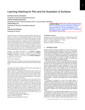
Learning Hatching for Pen-and-Ink Illustration of Surfaces(a) Estimated clusters usingour mixture-of-experts model(b) Learned labelingwith Joint Boosting(c) Learned labelingwith Joint Boosting CRF (d) Synthesized labelingfor another objectf1 a2f1 .73( I 3 ) .27(r)f1 .77(eb,3 ) .23( I 3 )f2 .54(kmax,1 ) .46(r )f2 .69(kmax,2 ) .31( I ,3 )f2 vf1 .59(eb,3 ) .41( (L · N )3 )f1 .88( a3 ) .12( (L · N )3 )f2 .63(ea,3 ) .37( (L · N ) ,3 )1:5f2 .45(kmax,2 ) .31( a ,3 ) .24(ea,3 )Fig. 3. Clustering orientations. The algorithm clusters stroke orientations according to different orientation rules. Each cluster specifies rules for hatching (f 1 )and cross-hatching (f 2 ) directions. Cluster labels are color-coded in the figure, with rules shown below. The cluster labels and the orientation rules are estimatedsimultaneously during learning. (a) Inferred cluster labels for an artist’s illustration of a screwdriver. (b) Output of the labeling step using the most likely labelsreturned by the Joint Boosting classifier alone. (c) Output of the labeling step using our full CRF model. (d) Synthesis of part labels for a novel object. Rules:In the legend, we show the corresponding orientation functions for each region. In all cases, the learned models use one to three features. Subscripts {1, 2, 3}indicate the scale used to compute the field. The operator rotates the field by 90 degrees in image-space. The orientation features used here are: maximumand minimum principal curvature directions (k max , k min ), PCA directions corresponding to first and second largest eigenvalue ( ea , e b ), fields aligned with ·N ( (L · N)). Features thatridges and valleys respectively ( r , v ), Lambertian image gradient ( I ), gradient of ambient occlusion ( a), and gradient of Larise as 3D vectors are projected to the image plane. See Appendix C for details.using a learning and clustering algorithm based on Mixtures-ofExperts (Section 5.1).Once the input pixels are classified, a pixel classifier is learnedusing Conditional Random Fields with unary terms based on JointBoost (Section 5.2). Finally, each real-valued property is learnedusing boosting for regression (Section 5.3). We use boosting techniques for classification and regression since we do not know inadvance which input features are the most important for differentstyles. Boosting can handle a large number of features, can select themost relevant features, and has a fast sequential learning algorithm.Synthesis. A hatching style is transferred to a target novel viewand/or object by first computing the features for each pixel, and thenapplying the learned mappings to compute the preceding hatchingproperties. A streamline synthesis algorithm [Hertzmann and Zorin2000] then places hatching strokes to match the synthesized properties. Examples of this process are shown in Figure 2.4.SYNTHESIS ALGORITHMThe algorithm for computing a pen-and-ink illustration of a viewof a 3D object is as follows. For each pixel of the target image,the features x and θ are first computed (Appendices B and C). Thesegment label and hatching level are each computed as a functionof the scalar features x, using image segmentation and recognitiontechniques. Given these segments, orientation fields for the targetimage are computed by interpolation of the orientation features θ.Then, the remaining hatching properties are computed by learningfunctions of the scalar features. Finally, a streamline synthesis algorithm [Hertzmann and Zorin 2000] renders strokes to match thesesynthesized properties. A streamline is terminated when it crossesan occlusion boundary, or the length grows past the value of the perpixel target stroke length l, or violates the target stroke spacing d.We now describe these steps in more detail. In Section 5, we willdescribe how the algorithm’s parameters are learned.4.1Segmentation and LabelingFor a given view of a 3D model, the algorithm first segments theimage into regions with different orientation rules and levels ofhatching. More precisely, given the feature set x for each pixel, thealgorithm computes the per-pixel segment labels c C and hatchinglevel h {0, 1, 2}. There are a few important considerations whenchoosing an appropriate segmentation and labeling algorithm. First,we do not know in advance which features in x are important, and sowe must use a method that can perform feature selection. Second,neighboring labels are highly correlated, and performing classification on each pixel independently yields noisy results (Figure 3).Hence, we use a Conditional Random Field (CRF) recognition algorithm, with JointBoost unary terms [Kalogerakis et al. 2010; Shottonet al. 2009; Torralba et al. 2007]. One such model is learned for segment labels c, and a second for hatching level h. Learning thesemodels is described in Section 5.2.The CRF objective function includes unary terms that assess theconsistency of pixels with labels, and pairwise terms that assess theconsistency between labels of neighboring pixels. Inferring segmentlabels based on the CRF model corresponds to minimizing thefollowing objective function. We have E1 (ci ; xi ) E2 (ci , cj ; xi , xj ),(1)E(c) ii,jwhere E1 is the unary term defined for each pixel i, E2 is thepairwise term defined for each pair of neighboring pixels {i, j },where j N (i) and N (i) is defined using the 8-neighborhood ofpixel i.The unary term evaluates a JointBoost classifier that, given thefeature set xi for pixel i, determines the probability P (ci xi ) foreach possible label ci . The unary term is thenE1 (ci ; x) log P (ci xi ).(2)ACM Transactions on Graphics, Vol. 31, No. 1, Article 1, Publication date: January 2012.

1:6 E. Kalogerakis et al.The mapping from features to probabilities P (ci xi ) is learned fromthe training data using the JointBoost algorithm [Torralba et al.2007].The pairwise energy term scores the compatibility of adjacentpixel labels ci and cj , given their features xi and xj . Let ei bea binary random variable representing if the pixel i belongs to aboundary of hatching region or not. We define a binary JointBoostclassifier that outputs the probability of boundaries of hatchingregions P (e x) and compute the pairwise term asE2 (ci , cj ; xi , xj ) · I (ci , cj ) · (log((P (ei xi ) P (ej xj ))) μ),(3)where , μ are the model parameters and I (ci , cj ) is an indicatorfunction that is 1 when ci cj and 0 when ci cj . The parameter controls the importance of the pairwise term while μ contributesto eliminating tiny segments and smoothing boundaries.Similarly, inferring hatching levels based on the CRF model corresponds to minimizing the following objective function. E1 (hi ; xi ) E2 (hi , hj ; xi , xj )(4)E(h) ii,jAs already mentioned, the unary term evaluates another JointBoostclassifier that, given the feature set xi for pixel i, determines theprobability P (hi xi ) for each hatching level h {0, 1, 2}. The pairwise term is also defined asE2 (hi , hj ; xi , xj ) · I (hi , hj ) · (log((P (ei xi ) P (ej xj ))) μ)(5)with the same values for the parameters of , μ as earlier.The most probable labeling is the one that minimizes the CRFobjective function E(c) and E(h), given their learned parameters.The CRFs are optimized using alpha-expansion graph-cuts [Boykovet al. 2001]. Details of learning the JointBoost classifiers and , μare given in Section 5.2.4.24.3Once the per-pixel segment labels c and hatching levels h are computed, the per-pixel orientations φ1 and φ2 are computed. The number of orientations to be synthesized is determined by h. When h 0(no hatching), no orientations are produced. When h 1 (singlehatching), only φ1 is computed and, when h 2 (cross-hatching),φ2 is also computed.Orientations are computed by regression on a subset of the orientation features θ for each pixel. Each cluster c may use a differentsubset of features. The features used by a segment are indexed by avector σ , that is, the features’ indices are σ (1), σ (2), . . . , σ (k). Eachorientation feature represents an orientation field in image space,such as the image projection of principal curvature directions. Inorder to respect 2-symmetries in orientation, a single orientation θis transformed to a vector as(6)The output orientation function is expressed as a weighted sum ofselected orientation features. We have wσ (k) vσ (k) ,(7)f (θ; w) kwhere σ (k) represents the index to the k-th orientation feature inthe subset of selected orientation features, vσ (k) is its vector representation, and w is a vector of weight parameters. There is anorientation function f (θ; wc,1 ) for each label c C and, if theACM Transactions on Graphics, Vol. 31, No. 1, Article 1, Publication date: January 2012.Computing Real-Valued PropertiesThe remaining hatching properties are real-valued quantities. Let ybe a feature to be synthesized on a pixel with feature set x. We usemultiplicative models of the form αk ak xσ (k) bk ,(8)y kwhere xσ (k) is the index to the k-th scalar feature from x. The useof a multiplicative model is inspired by Goodwin et al. [2007], whopropose a model for stroke thickness that can be approximated by aproduct of radial curvature and inverse depth. The model is learnedin the logarithmic domain, which reduces the problem to learningthe weighted sum. log(y) (9)αk log ak xσ (k) bkkLearning the parameters αk , ak , bk , σ (k) is again performed usinggradient-based boosting [Zemel and Pitassi 2001], as described inSection 5.3.5.LEARNINGWe now describe how to learn the parameters of the functions usedin the synthesis algorithm described in the previous section.5.1Computing Orientationsv [cos(2θ ), sin(2θ )]T .class contains cross-hatching regions, it has an additional orientation function f (θ; wc,2 ) for determining the cross-hatching directions. The resulting vector is computed to an image-space angle asφ atan2(y, x)/2.The weights w and feature selection σ are learned by the gradientbased boosting for regression algorithm of Zemel and Pitassi [2001].The learning of the parameters and the feature selection is describedin Section 5.1.Learning Segmentation and OrientationFunctionsIn our model, the hatching orientation for a single-hatching pixelis computed by first assigning the pixel to a cluster c, and thenapplying the orientation function f (θ; wc ) for that cluster. If weknew the clustering in advance, then it would be straightforwardto learn the parameters wc for each pixel. However, neither thecluster labels nor the parameters wc are present in the training data.In order to solve this problem, we develop a technique inspiredby Expectation-Maximization for Mixtures-of-Experts [Jordan andJacobs 1994], but specialized to handle the particular issues ofhatching.The input to this step is a set of pixels from the source illustration with their corresponding orientation feature set θ i , trainingorientations φi , and training hatching levels hi . Pixels containingintersections of strokes or no strokes are not used. Each cluster cmay contain either single-hatching or cross-hatching. Single-hatchclusters have a single orientation function (Eq. (7)), with unknownparameters wc1 . Clusters with cross-hatches have two subclusters,each with an orientation function with unknown parameters wc1 andwc2 . The two orientation functions are not constrained to producedirections orthogonal to each other. Every source pixel must belong to one of the top-level clusters, and every pixel belonging to across-hatching cluster must belong to one of its subclusters.For each training pixel i, we define a labeling probability γicindicating the probability that pixel i lies in top-level cluster c,such that c γic 1. Also, for each top-level cluster, we define a

Learning Hatching for Pen-and-Ink Illustration of Surfacessubcluster probability βicj , where j {1, 2}, such that βic1 βic2 1. The probability βicj measures how likely the stroke orientationat pixel i corresponds to a hatching or cross-hatching dire

pen-and-ink illustration of a 3D object, and learn a model of the artist’s style that maps from input features of the 3D object to target hatching properties. This model can then be applied to synthesize renderings of new views and new 3D objects. Shortly we present an overview o