Transcription
Improved Techniques for Training GANsTim Salimanstim@openai.comIan Goodfellowian@openai.comWojciech Zarembawoj@openai.comAlec Radfordalec@openai.comVicki Cheungvicki@openai.comXi Chenpeter@openai.comAbstractWe present a variety of new architectural features and training procedures that weapply to the generative adversarial networks (GANs) framework. Using our newtechniques, we achieve state-of-the-art results in semi-supervised classification onMNIST, CIFAR-10 and SVHN. The generated images are of high quality as confirmed by a visual Turing test: our model generates MNIST samples that humanscannot distinguish from real data, and CIFAR-10 samples that yield a human errorrate of 21.3%. We also present ImageNet samples with unprecedented resolutionand show that our methods enable the model to learn recognizable features ofImageNet classes.1IntroductionGenerative adversarial networks [1] (GANs) are a class of methods for learning generative modelsbased on game theory. The goal of GANs is to train a generator network G(z; θ (G) ) that producessamples from the data distribution, pdata (x), by transforming vectors of noise z as x G(z; θ (G) ).The training signal for G is provided by a discriminator network D(x) that is trained to distinguishsamples from the generator distribution pmodel (x) from real data. The generator network G in turnis then trained to fool the discriminator into accepting its outputs as being real.Recent applications of GANs have shown that they can produce excellent samples [2, 3]. However,training GANs requires finding a Nash equilibrium of a non-convex game with continuous, highdimensional parameters. GANs are typically trained using gradient descent techniques that aredesigned to find a low value of a cost function, rather than to find the Nash equilibrium of a game.When used to seek for a Nash equilibrium, these algorithms may fail to converge [4].In this work, we introduce several techniques intended to encourage convergence of the GANs game.These techniques are motivated by a heuristic understanding of the non-convergence problem. Theylead to improved semi-supervised learning peformance and improved sample generation. We hopethat some of them may form the basis for future work, providing formal guarantees of convergence.All code and hyperparameters may be found at https://github.com/openai/improved-gan.2Related workSeveral recent papers focus on improving the stability of training and the resulting perceptual qualityof GAN samples [2, 3, 5, 6]. We build on some of these techniques in this work. For instance, weuse some of the “DCGAN” architectural innovations proposed in Radford et al. [3], as discussedbelow.One of our proposed techniques, feature matching, discussed in Sec. 3.1, is similar in spirit toapproaches that use maximum mean discrepancy [7, 8, 9] to train generator networks [10, 11].30th Conference on Neural Information Processing Systems (NIPS 2016), Barcelona, Spain.
Another of our proposed techniques, minibatch features, is based in part on ideas used for batchnormalization [12], while our proposed virtual batch normalization is a direct extension of batchnormalization.One of the primary goals of this work is to improve the effectiveness of generative adversarialnetworks for semi-supervised learning (improving the performance of a supervised task, in this case,classification, by learning on additional unlabeled examples). Like many deep generative models,GANs have previously been applied to semi-supervised learning [13, 14], and our work can be seenas a continuation and refinement of this effort. In concurrent work, Odena [15] proposes to extendGANs to predict image labels like we do in Section 5, but without our feature matching extension(Section 3.1) which we found to be critical for obtaining state-of-the-art performance.3Toward Convergent GAN TrainingTraining GANs consists in finding a Nash equilibrium to a two-player non-cooperative game.Each player wishes to minimize its own cost function, J (D) (θ (D) , θ (G) ) for the discriminator andJ (G) (θ (D) , θ (G) ) for the generator. A Nash equilibirum is a point (θ (D) , θ (G) ) such that J (D) is at aminimum with respect to θ (D) and J (G) is at a minimum with respect to θ (G) . Unfortunately, finding Nash equilibria is a very difficult problem. Algorithms exist for specialized cases, but we are notaware of any that are feasible to apply to the GAN game, where the cost functions are non-convex,the parameters are continuous, and the parameter space is extremely high-dimensional.The idea that a Nash equilibrium occurs when each player has minimal cost seems to intuitively motivate the idea of using traditional gradient-based minimization techniques to minimize each player’scost simultaneously. Unfortunately, a modification to θ (D) that reduces J (D) can increase J (G) , anda modification to θ (G) that reduces J (G) can increase J (D) . Gradient descent thus fails to convergefor many games. For example, when one player minimizes xy with respect to x and another playerminimizes xy with respect to y, gradient descent enters a stable orbit, rather than converging tox y 0, the desired equilibrium point [16]. Previous approaches to GAN training have thusapplied gradient descent on each player’s cost simultaneously, despite the lack of guarantee that thisprocedure will converge. We introduce the following techniques that are heuristically motivated toencourage convergence:3.1Feature matchingFeature matching addresses the instability of GANs by specifying a new objective for the generatorthat prevents it from overtraining on the current discriminator. Instead of directly maximizing theoutput of the discriminator, the new objective requires the generator to generate data that matchesthe statistics of the real data, where we use the discriminator only to specify the statistics that wethink are worth matching. Specifically, we train the generator to match the expected value of thefeatures on an intermediate layer of the discriminator. This is a natural choice of statistics for thegenerator to match, since by training the discriminator we ask it to find those features that are mostdiscriminative of real data versus data generated by the current model.Letting f (x) denote activations on an intermediate layer of the discriminator, our new objective forthe generator is defined as: Ex pdata f (x) Ez pz (z) f (G(z)) 22 . The discriminator, and hencef (x), are trained in the usual way. As with regular GAN training, the objective has a fixed pointwhere G exactly matches the distribution of training data. We have no guarantee of reaching thisfixed point in practice, but our empirical results indicate that feature matching is indeed effective insituations where regular GAN becomes unstable.3.2Minibatch discriminationOne of the main failure modes for GAN is for the generator to collapse to a parameter setting whereit always emits the same point. When collapse to a single mode is imminent, the gradient of thediscriminator may point in similar directions for many similar points. Because the discriminatorprocesses each example independently, there is no coordination between its gradients, and thus nomechanism to tell the outputs of the generator to become more dissimilar to each other. Instead,all outputs race toward a single point that the discriminator currently believes is highly realistic.After collapse has occurred, the discriminator learns that this single point comes from the generator,but gradient descent is unable to separate the identical outputs. The gradients of the discriminator2
then push the single point produced by the generator around space forever, and the algorithm cannotconverge to a distribution with the correct amount of entropy. An obvious strategy to avoid this typeof failure is to allow the discriminator to look at multiple data examples in combination, and performwhat we call minibatch discrimination.The concept of minibatch discrimination is quite general: any discriminator model that looksat multiple examples in combination, rather than in isolation, could potentially help avoid collapse of the generator. In fact, the successful application of batch normalization in the discriminator by Radford et al. [3] is well explained from this perspective. So far, however, wehave restricted our experiments to models that explicitly aim to identify generator samples thatare particularly close together. One successful specification for modelling the closeness betweenexamples in a minibatch is as follows: Let f (xi ) RA denote a vector of features for input xi , produced by some intermediate layer in the discriminator. We then multiply the vectorf (xi ) by a tensor T RA B C , which results in a matrix Mi RB C . We then computethe L1 -distance between the rows of the resulting matrix Mi across samples i {1, 2, . . . , n}and apply a negative exponential (Fig. 1): cb (xi , xj ) exp( Mi,b Mj,b L1 ) R.The output o(xi ) for this minibatch layer for a sample xiis then defined as the sum of the cb (xi , xj )’s to all othersamples:nXo(xi )b cb (xi , xj ) Rj 1hio(xi ) o(xi )1 , o(xi )2 , . . . , o(xi )B RBo(X) Rn BNext, we concatenate the output o(xi ) of the minibatchlayer with the intermediate features f (xi ) that were its Figure 1: Figure sketches how miniinput, and we feed the result into the next layer of the batch discrimination works. Featuresdiscriminator. We compute these minibatch features sep- f (xi ) from sample xi are multipliedarately for samples from the generator and from the train- through a tensor T , and cross-sampleing data. As before, the discriminator is still required to distance is computed.output a single number for each example indicating howlikely it is to come from the training data: The task of the discriminator is thus effectively still toclassify single examples as real data or generated data, but it is now able to use the other examples inthe minibatch as side information. Minibatch discrimination allows us to generate visually appealingsamples very quickly, and in this regard it is superior to feature matching (Section 6). Interestingly,however, feature matching was found to work much better if the goal is to obtain a strong classifierusing the approach to semi-supervised learning described in Section 5.3.3Historical averagingPtWhen applying this technique, we modify each player’s cost to include a term θ 1t i 1 θ[i] 2 ,where θ[i] is the value of the parameters at past time i. The historical average of the parameters canbe updated in an online fashion so this learning rule scales well to long time series. This approach isloosely inspired by the fictitious play [17] algorithm that can find equilibria in other kinds of games.We found that our approach was able to find equilibria of low-dimensional, continuous non-convexgames, such as the minimax game with one player controlling x, the other player controlling y, andvalue function (f (x) 1)(y 1), where f (x) x for x 0 and f (x) x2 otherwise. Forthese same toy games, gradient descent fails by going into extended orbits that do not approach theequilibrium point.3.4One-sided label smoothingLabel smoothing, a technique from the 1980s recently independently re-discovered by Szegedy et.al [18], replaces the 0 and 1 targets for a classifier with smoothed values, like .9 or .1, and wasrecently shown to reduce the vulnerability of neural networks to adversarial examples [19].Replacing positive classification targets with α and negative targets with β, the optimal discriminatordata (x) βpmodel (x)becomes D(x) αppdata(x) pmodel (x) . The presence of pmodel in the numerator is problematicbecause, in areas where pdata is approximately zero and pmodel is large, erroneous samples from3
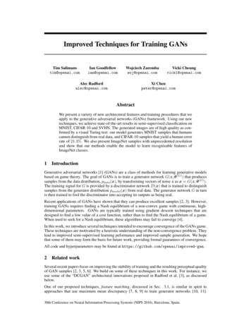
pmodel have no incentive to move nearer to the data. We therefore smooth only the positive labels toα, leaving negative labels set to 0.3.5Virtual batch normalizationBatch normalization greatly improves optimization of neural networks, and was shown to be highlyeffective for DCGANs [3]. However, it causes the output of a neural network for an input examplex to be highly dependent on several other inputs x0 in the same minibatch. To avoid this problemwe introduce virtual batch normalization (VBN), in which each example x is normalized based onthe statistics collected on a reference batch of examples that are chosen once and fixed at the startof training, and on x itself. The reference batch is normalized using only its own statistics. VBN iscomputationally expensive because it requires running forward propagation on two minibatches ofdata, so we use it only in the generator network.4Assessment of image qualityGenerative adversarial networks lack an objective function, which makes it difficult tocompare performance of different models.One intuitive metric of performance can beobtained by having human annotators judge the visual quality of samples [2].Weautomate this process using Amazon Mechanical Turk (MTurk), using the web interface in figure Fig. 2 (live at minibatch/), which we use to ask annotators to distinguish between generated dataand real data. The resulting quality assessments of our models are described in Section 6.Figure 2: Web interface given to annotators. Annotators are asked to distinguish computer generated images fromreal ones.A downside of using human annotators is that the metricvaries depending on the setup of the task and the motivation of the annotators. We also find that results changedrastically when we give annotators feedback about theirmistakes: By learning from such feedback, annotators arebetter able to point out the flaws in generated images, giving a more pessimistic quality assessment. The left column of Fig. 2 presents a screen from the annotation process, while the right column shows how we inform annotators about their mistakes.As an alternative to human annotators, we propose an automatic method to evaluate samples, whichwe find to correlate well with human evaluation: We apply the Inception model1 [20] to everygenerated image to get the conditional label distribution p(y x). Images that contain meaningfulobjects should have a conditional label distribution p(y x)with low entropy. Moreover, we expectRthe model to generate varied images, so the marginal p(y x G(z))dz should have high entropy.Combining these two requirements, the metric that we propose is: exp(Ex KL(p(y x) p(y))), wherewe exponentiate results so the values are easier to compare. Our Inception score is closely relatedto the objective used for training generative models in CatGAN [14]: Although we had less successusing such an objective for training, we find it is a good metric for evaluation that correlates verywell with human judgment. We find that it’s important to evaluate the metric on a large enoughnumber of samples (i.e. 50k) as part of this metric measures diversity.5Semi-supervised learningConsider a standard classifier for classifying a data point x into one of K possible classes. Sucha model takes in x as input and outputs a K-dimensional vector of logits {l1 , . . . , lK }, that canexp(lj )be turned into class probabilities by applying the softmax: pmodel (y j x) PK exp(l. Ink)k 1supervised learning, such a model is then trained by minimizing the cross-entropy between theobserved labels and the model predictive distribution pmodel (y x).1We use the pretrained Inception model from et/inception-2015-12-05.tgz. Code to compute the Inception score with this model will be madeavailable by the time of publication.4
We can do semi-supervised learning with any standard classifier by simply adding samples fromthe GAN generator G to our data set, labeling them with a new “generated” class y K 1, andcorrespondingly increasing the dimension of our classifier output from K to K 1. We may thenuse pmodel (y K 1 x) to supply the probability that x is fake, corresponding to 1 D(x) inthe original GAN framework. We can now also learn from unlabeled data, as long as we know thatit corresponds to one of the K classes of real data by maximizing log pmodel (y {1, . . . , K} x).Assuming half of our data set consists of real data and half of it is generated (this is arbitrary), ourloss function for training the classifier then becomesL Ex,y pdata (x,y) [log pmodel (y x)] Ex G [log pmodel (y K 1 x)] Lsupervised Lunsupervised , whereLsupervised Ex,y pdata (x,y) log pmodel (y x, y K 1)Lunsupervised {Ex pdata (x) log[1 pmodel (y K 1 x)] Ex G log[pmodel (y K 1 x)]},where we have decomposed the total cross-entropy loss into our standard supervised loss functionLsupervised (the negative log probability of the label, given that the data is real) and an unsupervisedloss Lunsupervised which is in fact the standard GAN game-value as becomes evident when we substitute D(x) 1 pmodel (y K 1 x) into the expression:Lunsupervised {Ex pdata (x) log D(x) Ez noise log(1 D(G(z)))}.The optimal solution for minimizing both Lsupervised and Lunsupervised is to haveexp[lj (x)] c(x)p(y j, x) j K 1 and exp[lK 1 (x)] c(x)pG (x) for some undetermined scaling function c(x). The unsupervised loss is thus consistent with the supervised loss inthe sense of Sutskever et al. [13], and we can hope to better estimate this optimal solution fromthe data by minimizing these two loss functions jointly. In practice, Lunsupervised will only help ifit is not trivial to minimize for our classifier and we thus need to train G to approximate the datadistribution. One way to do this is by training G to minimize the GAN game-value, using thediscriminator D defined by our classifier. This approach introduces an interaction between G andour classifier that we do not fully understand yet, but empirically we find that optimizing G usingfeature matching GAN works very well for semi-supervised learning, while training G using GANwith minibatch discrimination does not work at all. Here we present our empirical results using thisapproach; developing a full theoretical understanding of the interaction between D and G using thisapproach is left for future work.Finally, note that our classifier with K 1 outputs is over-parameterized: subtracting a generalfunction f (x) from each output logit, i.e. setting lj (x) lj (x) f (x) j, does not change theoutput of the softmax. This means we may equivalently fix lK 1 (x) 0 x, in which case Lsupervisedbecomes the standard supervised loss function of our originalclassifier with K classes, and ourPKZ(x)discriminator D is given by D(x) Z(x) 1, where Z(x) k 1 exp[lk (x)].5.1Importance of labels for image qualityBesides achieving state-of-the-art results in semi-supervised learning, the approach described abovealso has the surprising effect of improving the quality of generated images as judged by humanannotators. The reason appears to be that the human visual system is strongly attuned to imagestatistics that can help infer what class of object an image represents, while it is presumably lesssensitive to local statistics that are less important for interpretation of the image. This is supportedby the high correlation we find between the quality reported by human annotators and the Inceptionscore we developed in Section 4, which is explicitly constructed to measure the “objectness” of agenerated image. By having the discriminator D classify the object shown in the image, we bias it todevelop an internal representation that puts emphasis on the same features humans emphasize. Thiseffect can be understood as a method for transfer learning, and could potentially be applied muchmore broadly. We leave further exploration of this possibility for future work.5
6ExperimentsWe performed semi-supervised experiments on MNIST, CIFAR-10 and SVHN, and sample generation experiments on MNIST, CIFAR-10, SVHN and ImageNet. We provide code to reproduce themajority of our experiments.6.1MNISTThe MNIST dataset contains 60, 000 labeledimages of digits. We perform semi-supervisedtraining with a small randomly picked fractionof these, considering setups with 20, 50, 100,and 200 labeled examples. Results are averagedover 10 random subsets of labeled data, eachchosen to have a balanced number of examplesfrom each class. The remaining training imagesare provided without labels. Our networks have5 hidden layers each. We use weight normalization [21] and add Gaussian noise to the output Figure 3: (Left) samples generated by model durof each layer of the discriminator. Table 1 sum- ing semi-supervised training. Samples can bemarizes our results.clearly distinguished from images coming fromSamples generated by the generator during MNIST dataset. (Right) Samples generated withsemi-supervised learning using feature match- minibatch discrimination. Samples are coming (Section 3.1) do not look visually appealing pletely indistinguishable from dataset images.(left Fig. 3). By using minibatch discriminationinstead (Section 3.2) we can improve their visual quality. On MTurk, annotators were able to distinguish samples in 52.4% of cases (2000 votes total), where 50% would be obtained by randomguessing. Similarly, researchers in our institution were not able to find any artifacts that would allow them to distinguish samples. However, semi-supervised learning with minibatch discriminationdoes not produce as good a classifier as does feature matching.Model20DGN [22]Virtual Adversarial [23]CatGAN [14]Skip Deep Generative Model [24]Ladder network [25]Auxiliary Deep Generative Model [24]Our modelEnsemble of 10 of our modelsNumber of incorrectly predicted test examplesfor a given number of labeled samples501001677 4521134 445221 136142 96333 14212191 10132 7106 3796 293 6.586 5.620090 4.281 4.3Table 1: Number of incorrectly classified test examples for the semi-supervised setting on permutation invariant MNIST. Results are averaged over 10 seeds.6.2CIFAR-10Model1000Ladder network [25]CatGAN [14]Our modelEnsemble of 10 of our models21.83 2.0119.22 0.54Test error rate fora given number of labeled samples2000400019.61 2.0917.25 0.6620.40 0.4719.58 0.4618.63 2.3215.59 0.47800017.72 1.8214.87 0.89Table 2: Test error on semi-supervised CIFAR-10. Results are averaged over 10 splits of data.CIFAR-10 is a small, well studied dataset of 32 32 natural images. We use this data set to studysemi-supervised learning, as well as to examine the visual quality of samples that can be achieved.For the discriminator in our GAN we use a 9 layer deep convolutional network with dropout andweight normalization. The generator is a 4 layer deep CNN with batch normalization. Table 2summarizes our results on the semi-supervised learning task.6
Figure 4: Samples generated during semi-supervised training on CIFAR-10 with feature matching(Section 3.1, left) and minibatch discrimination (Section 3.2, right).When presented with 50% real and 50% fake data generated by our best CIFAR-10 model, MTurkusers correctly categorized 78.7% of images correctly. However, MTurk users may not be sufficiently familiar with CIFAR-10 images or sufficiently motivated; we ourselves were able to categorize images with 95% accuracy. We validated the Inception score described above by observingthat MTurk accuracy drops to 71.4% when the data is filtered by using only the top 1% of samplesaccording to the Inception score. We performed a series of ablation experiments to demonstrate thatour proposed techniques improve the Inception score, presented in Table 3. We also present imagesfor these ablation experiments—in our opinion, the Inception score correlates well with our subjective judgment of image quality. Samples from the dataset achieve the highest value. All the modelsthat even partially collapse have relatively low scores. We caution that the Inception score should beused as a rough guide to evaluate models that were trained via some independent criterion; directlyoptimizing Inception score will lead to the generation of adversarial examples [26].SamplesModelScore std.Real data11.24 .12Our methods8.09 .07-VBN BN7.54 .07-L HA6.86 .06-LS6.83 .06-L4.36 .04-MBF3.87 .03Table 3: Table of Inception scores for samples generated by various models for 50, 000 images.Score highly correlates with human judgment, and the best score is achieved for natural images.Models that generate collapsed samples have relatively low score. This metric allows us to avoidrelying on human evaluations. “Our methods” includes all the techniques described in this work,except for feature matching and historical averaging. The remaining experiments are ablation experiments showing that our techniques are effective. “-VBN BN” replaces the VBN in the generatorwith BN, as in DCGANs. This causes a small decrease in sample quality on CIFAR. VBN is moreimportant for ImageNet. “-L HA” removes the labels from the training process, and adds historicalaveraging to compensate. HA makes it possible to still generate some recognizable objects. WithoutHA, sample quality is considerably reduced (see ”-L”). “-LS” removes label smoothing and incurs anoticeable drop in performance relative to “our methods.” “-MBF” removes the minibatch featuresand incurs a very large drop in performance, greater even than the drop resulting from removing thelabels. Adding HA cannot prevent this problem.6.3SVHNFor the SVHN data set, we used the same architecture and experimental setup as for CIFAR-10.Figure 5 compares against the previous state-of-the-art, where it should be noted that the model7
of [24] is not convolutional, but does use an additional data set of 531131 unlabeled examples. Theother methods, including ours, are convolutional and do not use this data.ModelPercentage of incorrectly predicted test examplesfor a given number of labeled samples50010002000Virtual Adversarial [23]Stacked What-Where Auto-Encoder [27]DCGAN [3]Skip Deep Generative Model [24]Our modelEnsemble of 10 of our models24.6323.5622.4816.61 0.248.11 1.35.88 1.018.44 4.86.16 0.58Figure 5: (Left) Error rate on SVHN. (Right) Samples from the generator for SVHN.6.4ImageNetWe tested our techniques on a dataset of unprecedented scale: 128 128 images from theILSVRC2012 dataset with 1,000 categories. To our knowledge, no previous publication has applied a generative model to a dataset with both this large of a resolution and this large a numberof object classes. The large number of object classes is particularly challenging for GANs due totheir tendency to underestimate the entropy in the distribution. We extensively modified a publiclyavailable implementation of DCGANs2 using TensorFlow [28] to achieve high performance, usinga multi-GPU implementation. DCGANs without modification learn some basic image statistics andgenerate contiguous shapes with somewhat natural color and texture but do not learn any objects.Using the techniques described in this paper, GANs learn to generate objects that resemble animals,but with incorrect anatomy. Results are shown in Fig. 6.Figure 6: Samples generated from the ImageNet dataset. (Left) Samples generated by a DCGAN.(Right) Samples generated using the techniques proposed in this work. The new techniques enableGANs to learn recognizable features of animals, such as fur, eyes, and noses, but these features arenot correctly combined to form an animal with realistic anatomical structure.7ConclusionGenerative adversarial networks are a promising class of generative models that has so far beenheld back by unstable training and by the lack of a proper evaluation metric. This work presentspartial solutions to both of these problems. We propose several techniques to stabilize trainingthat allow us to train models that were previously untrainable. Moreover, our proposed evaluationmetric (the Inception score) gives us a basis for comparing the quality of these models. We applyour techniques to the problem of semi-supervised learning, achieving state-of-the-art results on anumber of different data sets in computer vision. The contributions made in this work are of apractical nature; we hope to develop a more rigorous theoretical understanding in future w8
References[1] Ian Goodfellow, Jean Pouget-Abadie, Mehdi Mirza, et al. Generative adversarial nets. In NIPS, 2014.[2] Emily Denton, Soumith Chintala, Arthur Szlam, and Rob Fergus. Deep generative image models using alaplacian pyramid of adversarial networks. arXiv preprint arXiv:1506.05751, 2015.[3] Alec Radford, Luke Metz, and Soumith Chintala. Unsupervised representation learning with deep convolutional generative adversarial networks. arXiv preprint arXiv:1511.06434, 2015.[4] Ian J Goodfellow. On distinguishability criteria for estimating generative models. arXiv preprintarXiv:1412.6515, 2014.[5] Daniel Jiwoong Im, Chris Dongjoo Kim, Hui Jiang, and Roland Memisevic. Generating images withrecurrent adversarial networks. arXiv preprint arXiv:1602.05110, 2016.[6] Donggeun Yoo, Namil Kim, Sunggyun Park, Anthony S Paek, and In So Kweon. Pixel-level domaintransfer. arXiv preprint arXiv:1603.07442, 2016.[7] Arthur Gretton, Olivier Bousquet, Alex Smola, and Bernhard Schölkopf. Measuring statistical dependence with hilbert-schmidt norms. In Algorithmic learning theory, pages 63–77. Springer, 2005.[8] Kenji Fukumizu, Arthur Gretton, Xiaohai Sun, and Bernhard Schölkopf. Kernel measures of conditionaldependence. In NIPS, volume 20, pages 489–496, 2007.[9] Alex Smola, Arthur Gretton, Le Song, and Bernhard Schölkopf. A hilbert space embedding for distributions. In Algorithmic learning theory, pages 13–31. Springer, 2007.[10] Yujia Li, Kevin Swersky, and Richard S. Zemel. Generative moment matching networks. CoRR,abs/1502.02761, 2015.[11] Gintare Karolina Dziugaite, Daniel M Roy, and Zo
One of our proposed techniques, feature matching, discussed in Sec. 3.1, is similar in spirit to approaches that use maximum mean discrepancy [7, 8, 9] to train generator networks [10, 11]. 30th Conference on Neural Info