WIXLIB

ECE 5520 Fall 20098Lecture 1Today: (1) Syllabus (2) Intro to Digital Communications1Class OrganizationTextbook Few textbooks cover solely digital communications (without analog) in an introductory communications course. But graduates today will almost always encounter / be developing solely digital communicationsystems. So half of most textbooks are useless; and that the other half is sparse and needs supplemental material.For example, the past text was the ‘standard’ text in the area for an undergraduate course, Proakis & Salehi,J.G. Proakis and M. Salehi, Communication Systems Engineering, 2nd edition, Prentice Hall, 2001. Studentsdidn’t like that I had so many supplemental readings. This year’s text covers primarily digital communications,and does it in depth. Finally, I find it to be very well-written. And, there are few options in this area. I willprovide additional readings solely to provide another presentation style or fit another learning style. Unlessspecified, these are optional.Lecture Notes I type my lecture notes. I have taught ECE 5520 previously and have my lecture notes frompast years. I’m constantly updating my notes, even up to the lecture time. These can be available to you atlecture, and/or after lecture online. However, you must accept these conditions:1. Taking notes is important: I find most learning requires some writing on your part, not just watching.Please take your own notes.2. My written notes do not and cannot reflect everything said during lecture: I answer questionsand understand your perspective better after hearing your questions, and I try to tailor my approachduring the lecture. If I didn’t, you could just watch a recording!2IntroductionA digital communication system conveys discrete-time, discrete-valued information across a physical channel.Information sources might include audio, video, text, or data. They might be continuous-time (analog) signals(audio, images) and even 1-D or 2-D. Or, they may already be digital (discrete-time, discrete-valued). Ourobject is to convey the signals or data to another place (or time) with as faithful representation as possible.In this section we talk about what we’ll cover in this class, and more importantly, what we won’t cover.2.1”Executive Summary”Here is the one sentence version: We will study how to efficiently encode digital data on a noisy, bandwidthlimited analog medium, so that decoding the data (i.e., reception) at a receiver is simple, efficient, and highfidelity.The keys points stuffed into that one sentence are:1. Digital information on an analog medium: We can send waveforms, i.e., real-valued, continuous-timefunctions, on the channel (medium). These waveforms are from a discrete set of possible waveforms.What set of waveforms should we use? Why?

ECE 5520 Fall 200992. Decoding the data: When receiving a signal (a function) in noise, none of the original waveforms willmatch exactly. How do you make a decision about which waveform was sent?3. What makes a receiver difficult to realize? What choices of waveforms make a receiver simpler to implement? What techniques are used in a receiver to compensate?4. Efficiency, Bandwidth, and Fidelity: Fidelity is the correctness of the received data (i.e., the opposite oferror rate). What is the tradeoff between energy, bandwidth, and fidelity? We all want high fidelity, andlow energy consumption and bandwidth usage (the costs of our communication system).You can look at this like an impedance matching problem from circuits. You want, for power efficiency, tohave the source impedance match the destination impedance. In digital comm, this means that we want ourwaveform choices to match the channel and receiver to maximize the efficiency of the communication system.2.2Why not Analog?The previous text used for this course, by Proakis & Salehi, has an extensive analysis and study of analogcommunication systems, such as radio and television broadcasting (Chapter 3). In the recent past, this coursewould study both analog and digital communication systems. Analog systems still exist and will continue toexist; however, development of new systems will almost certainly be of digital communication systems. Why? Fidelity Energy: transmit power, and device power consumption Bandwidth efficiency: due to coding gains Moore’s Law is decreasing device costs for digital hardware Increasing need for digital information More powerful information security2.3Networking StackIn this course, we study digital communications from bits to bits. That is, we study how to take ones and zerosfrom a transmitter, send them through a medium, and then (hopefully) correctly identify the same ones andzeros at the receiver. There’s a lot more than this to the digital communication systems which you use on adaily basis (e.g., iPhone, WiFi, Bluetooth, wireless keyboard, wireless car key).To manage complexity, we (engineers) don’t try to build a system to do everything all at once. We typicallystart with an application, and we build a layered network to handle the application. The 7-layer OSI stack,which you would study in a CS computer networking class, is as follows: Application Presentation (*) Session (*) Transport Network

10ECE 5520 Fall 2009 Link Layer Physical (PHY) Layer(Note that there is also a 5-layer model in which * layers are considered as part of the application layer.) ECE5520 is part of the bottom layer, the physical layer. In fact, the physical layer has much more detail. It isprimarily divided into: Multiple Access Control (MAC) Encoding Channel / MediumWe can control the MAC and the encoding chosen for a digital communication.2.4Channels and MediaWe can chose from a few media, but we largely can’t change the properties of the medium (although there areexceptions). Here are some media: EM Spectra: (anything above 0 Hz) Radio, Microwave, mm-wave bands, light Acoustic: ultrasound Transmission lines, waveguides, optical fiber, coaxial cable, wire pairs, . Disk (data storage applications)2.5Encoding / Decoding Block DiagramInformationSourceSourceEncoderOther coderDigital to AnalogConverterChannelDecoderModulatorAnalog to ationChannelDownconversionFigure 1: Block diagram of a single-user digital communication system, including (top) transmitter, (middle)channel, and (bottom) receiver.Notes: Information source comes from higher networking layers. It may be continuous or packetized. Source Encoding: Finding a compact digital representation for the data source. Includes sampling ofcontinuous-time signals, and quantization of continuous-valued signals. Also includes compression ofthose sources (lossy, or lossless). What are some compression methods that you’re familiar with? Wepresent an introduction to source encoding at the end of this course.

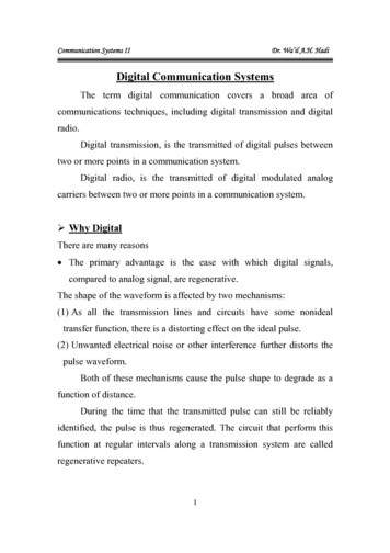
11ECE 5520 Fall 2009 Channel encoding refers to redundancy added to the signal such that any bit errors can be corrected.A channel decoder, because of the redundancy, can correct some bit errors. We will not study channelencoding, but it is a topic in the (ECE 6520) Coding Theory. Modulation refers to the digital-to-analog conversion which produces a continuous-time signal that can besent on the physical channel. It is analogous to impedance matching - proper matching of a modulation toa channel allows optimal information transfer, like impedance matching ensured optimal power transfer.Modulation and demodulation will be the main focus of this course. Channels: See above for examples. Typical models are additive noise, or linear filtering channel.Why do we do both source encoding (which compresses the signal as much as possible) and also channelencoding (which adds redundancy to the signal)? Because of Shannon’s source-channel coding separationtheorem. He showed that (given enough time) we can consider them separately without additional loss. Andseparation, like layering, reduces complexity to the designer.2.6ChannelsA channel can typically be modeled as a linear filter with the addition of noise. The noise comes from a varietyof sources, but predominantly:1. Thermal background noise: Due to the physics of living above 0 Kelvin. Well modeled as Gaussian, andwhite; thus it is referred to as additive white Gaussian noise (AWGN).2. Interference from other transmitted signals. These other transmitters whose signals we cannot completelycancel, we lump into the ‘interference’ category. These may result in non-Gaussian noise distribution, ornon-white noise spectral density.The linear filtering of the channel result from the physics and EM of the medium. For example, attenuation intelephone wires varies by frequency. Narrowband wireless channels experience fading that varies quickly as afunction of frequency. Wideband wireless channels display multipath, due to multiple time-delayed reflections,diffractions, and scattering of the signal off of the objects in the environment. All of these can be modeled aslinear filters.The filter may be constant, or time-invariant, if the medium, the TX and RX do not move or change.However, for mobile radio, the channel may change very quickly over time. Even for stationary TX and RX, inreal wireless channels, movement of cars, people, trees, etc. in the environment may change the channel slowlyover time.NoiseTransmittedSignalLTI Filterh(t)ReceivedSignalFigure 2: Linear filter and additive noise channel model.In this course, we will focus primarily on the AWGN channel, but we will mention what variations exist forparticular channels, and how they are addressed.

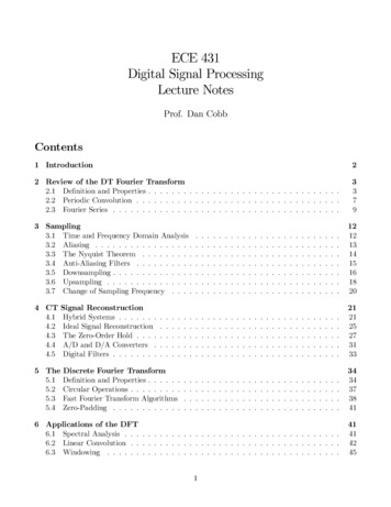
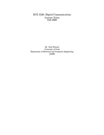
12ECE 5520 Fall 20092.7Topic: Random ProcessesRandom things in a communication system: Noise in the channel Signal (bits) Channel filtering, attenuation, and fading Device frequency, phase, and timing offsetsThese random signals often pass through LTI filters, and are sampled. We want to build the best receiverpossible despite the impediments. Optimal receiver design is something that we study using probability theory.We have to tolerate errors. Noise and attenuation of the channel will cause bit errors to be made by thedemodulator and even the channel decoder. This may be tolerated, or a higher layer networking protocol (eg.,TCP-IP) can determine that an error occurred and then re-request the data.2.8Topic: Frequency Domain RepresentationsTo fit as many signals as possible onto a channel, we often split the signals by frequency. The concept ofsharing a channel is called multiple access (MA). Separating signals by frequency band is called frequencydivision multiple access (FDMA). For the wireless channel, this is controlled by the FCC (in the US) and calledspectrum allocation. There is a tradeoff between frequency requirements and time requirements, which will bea major part of this course. The Fourier transform of our modulated, transmitted signal is used to show thatit meets the spectrum allocation limits of the FCC.2.9Topic: Orthogonality and Signal spacesTo show that signals sharing the same channel don’t interfere with each other, we need to show that they areorthogonal. This means, in short, that a receiver can uniquely separate them. Signals in different frequencybands are orthogonal.We can also employ multiple orthogonal signals in a single transmitter and receiver, in order to providemultiple independent means (dimensions) on which to modulate information. We will study orthogonal signals,and learn an algorithm to take an arbitrary set of signals and output a set of orthogonal signals with which torepresent them. We’ll use signal spaces to show graphically the results, as the example in Figure 36.M 8M 16Figure 3: Example signal space diagram for M -ary Phase Shift Keying, for (a) M 8 and (b) M 16. Eachpoint is a vector which can be used to send a 3 or 4 bit sequence.

13ECE 5520 Fall 20092.10Related classes1. Pre-requisites: (ECE 5510) Random Processes; (ECE 3500) Signals and Systems.2. Signal Processing: (ECE 5530): Digital Signal Processing3. Electromagnetics: EM Waves, (ECE 5320-5321) Microwave Engineering, (ECE 5324) Antenna Theory,(ECE 5411) Fiberoptic Systems4. Breadth: (ECE 5325) Wireless Communications5. Devices and Circuits: (ECE 3700) Fundamentals of Digital System Design, (ECE 5720) Analog IC Design6. Networking: (ECE 5780) Embedded System Design, (CS 5480) Computer Networks7. Advanced Classes: (ECE 6590) Software Radio, (ECE 6520) Information Theory and Coding, (ECE 6540):Estimation TheoryLecture 2Today: (1) Power, Energy, dB (2) Time-domain concepts (3) Bandwidth, Fourier TransformTwo of the biggest limitations in communications systems are (1) energy / power ; and (2) bandwidth. Today’slecture provides some tools to deal with power and energy, and starts the review of tools to analyze frequencycontent and bandwidth.3Power and EnergyRecall that energy is power times time. Use the units: energy is measured in Joules (J); power is measured inWatts (W) which is the same as Joules/second (J/sec). Also, recall that our standard in signals and systems isdefine our signals, such as x(t), as voltage signals (V). When we want to know the power of a signal we assumeit is being dissipated in a 1 Ohm resistor, so x(t) 2 is the power dissipated at time t (since power is equal tothe voltage squared divided by the resistance).A signal x(t) has energy defined asZE x(t) 2 dtFor some signals, E will be infinite because the signal is non-zero for an infinite duration of time (it is alwayson). These signals we call power signals and we compute their power as1P limT 2TThe signal with finite energy is called an energy signal.ZT T x(t) 2 dt

14ECE 5520 Fall 20093.1Discrete-Time SignalsIn this book, we refer to discrete samples of the sampled signal x as x(n). You may be more familiar with thex[n] notation. But, Matlab uses parentheses also; so we’ll follow the Rice text notation. Essentially, wheneveryou see a function of n (or k, l, m), it is a discrete-time function; whenever you see a function of t (or perhapsτ

A digital communication system conveys discrete-time, discrete-valued information across a physical channel. Information sources might include audio, video, text, or data. They might be continuous-time (analog) signals (audio, images) and even 1-D or 2-D. Or, they may already be