WIXLIB

2.3Holographic Principle for General SpacetimesGeneralize the statement in 2.2, we give the following statement:Holographic principle. Let A be the area of a connected (D 2)-dimensional spatial surface Γ. A (D 1) hypersuface Γ is bounded by Γ and is generated by one of the four nullcongruences orthogonal to Γ. Let S be the total entropy contained on Γ. If the expansion ofthe congruence is non-positive (measured in the direction away from Γ) at every point on Γ,Athen S 4G.Then it will be important to ask the question: which surfaces store the informationcontained in the entire space-time? Given a null hypersurface L, one should follow the geodesicgenerators of L in the direction of non-negative expansion. One can stop anytime, but onemust stop when the expansion becomes negative. This procedure is called projection. The(D-2)-dimensional spatial surface B spanned by the points where the projection is terminatedis called the screen of the projection. A preferred screen is the screen where the expansionvanishes on every point on it.Then we can write out the “standard” recipe of the whole process with the help of Penrosediagram:(1) Draw a Penrose diagram. Every point represents a (D-2)-sphere. Each diagonal linerepresents a light-cone. The two inequivalent light sheets can be represented by theascending and descending families of diagonal lines.(2) Pick one of the two light sheets {L}. Now the question is in which direction to projectalong the diagonal lines.(3) Identify the apparent horizons, i.e., hypersurfaces on which the expansion of the past orfuture light-cones vanishes. They will divide the space-time into normal, trapped, andanti-trapped regions. In each region, draw a wedge whose legs point in the direction ofnegative expansion of the cones.(4) On a given diagonal line (i.e., light-cone), project each point towards the tip of the localwedge, onto the nearest point (i.e., sphere) Bi where the direction of the tip flips, or ontothe boundary of space-time as the case may be.(5) Repeat for every line in the family. The surfaces Bi will form (preferred) screen-hypersurfaces.Take the Schwarszchild black hole as an example, the Penrose diagram of it is shown in figure3.To decied the wedge direction we calculate the expansion scalar θ µ k µ . The lightrays in Penrose diagram corresponds to vector field X . It is easy to see that at eventhorizon r rs , the expansion scalar θ is 0. The affine parameter both outside and inside thehorizon can be T , and T 0 when r rs . Following the focusing theorem, we can draw thelocal wedge in figure 3. Then we notice that the preferred screen is I .2.4Holographic Bound in Cosmological BackgroundWe can using the same method to prove the holographic bound in cosmology followingBousso’s provement [6]. One important difference is that this time the universe is changing with the scale factor a(t) which provides other possibilities.–6–

Figure 3. The Penrose diagram of the Schwarzschild black hole. The red dotted lines represent thelight sheets. The non-negative expansion of geodesics gives the the direction of the light sheets, thenthe event horizon becomes the preferred screenGiven region Γ, at the boundary Γ, we can construct four kinds of light rays, two of thempointing the past and two pointing the future, we call them 4 branches. In static spacetime,if Γ is convex, the outgoing branches always have positive expansion, but when consideringthe universe is expanding, it might be possible that outgoing branches also have negativeexpansion.The Bousso’s statement is as the following: from the boundary Γ construct all light sheetswhich have negative expansion as we move away. These light sheets may terminate at the tipof a cone or a caustic or even a boundary of the geometry. Bousso’s bound states that theAentropy passing through these light sheets is less that 4Gwhere A is the area of Γ.Suppose the spherical region Γ with boundary Γ radius R. Now consider the light-like surfaceL formed by past light rays from B toward the center of Γ.Now consider the entropy(particles)passing through L, apply the holographic principle to the case, we get the holographic principle in cosmology: the entropy passing through L never exceeds the area of the boundingsurface Γ.Assume a horizon has a size of RH as is shown in Fig. 4:(a) If R RH , the surface of L forms a light cone with its tip in the future of the singularityat t 0.(b) If R RH , then L is still a cone but with its tip at t 0.(c) if R RH , the surface is a truncated cone. (this won’t give any special result)Figure 4. The stucture of the light cone.–7–

In order to illustrate the statement more clearly, we draw the Penrose diagram andfollow the standard steps to find the preferred screen. Taking de Sitter space (inflation) asan example. A 4-dim de Sitter spacetime is defined like:ds2 dt2 e2Ht (dr2 r2 dΩ22 )(2.26)qwhere the Hubble parameter satisfy H Λ3 . This is the flat slice of de Sitter space, define:p1 H 2 χ2sinh(Ht) H 2 Ht r e sinh(Hτ )T H2Hpcosh(Ht) H 2 Ht1 H 2 χ2R r e cosh(Hτ )H2H(2.27)(2.28)It returns to standard formula of de Sitter solution:ds2 (1 H 2 χ2 )dτ 2 dχ2 χ2 dΩ22(1 H 2 χ2 )(2.29)The porcess of finding preferred screen is shown in Fig. 5.For a general FLRW metric, it can be written in conformal time τ :Figure 5. Penrose diagram for de Sitter space. The dS 4 spacelike slices would correspond to horizontal lines through the square. The diagonals are apparent horizons dividing the space-time into fourregions (a). The 2-spheres near past (future) infinity are trapped (anti-trapped); the spheres near thepoles are normal. It follows that de Sitter space can be projected onto past and future infinity (b),which are spacelike, optimal screen-hypersurfaces of (exponentially) infinite size. A more interestingscreen is obtained by applying the spacelike projection theorem to spheres near the particle horizonof an observer at χ 0 (a). By taking a limit, one can show that all information in the observableregion of de Sitter space can be projected onto the particle horizon, which is a null hypersurface ofconstant spatial area 4πH 2 (c).ds2 a2 (τ )(dτ 2 dχ2 r(χ)2 dΩ22 )(2.30)When χ r this metric returns to spatially flat FRW metric. r sin χ is the closed universeand r sinh χ is the open universe. The particle horizon isZ tdt0τ χ(t) χ τ (2.31)00 a(t )–8–

The general solution from the Freedmann equation is given by 2(1 3w)τ 1 3wa(τ ) 2(2.32)The apparent horizon is defined as geometrically as the spheres on which at least one pair oforthogonal null congruences have zero expansion. It can be read from Penrose diagram andis given by:2τ χ(2.33)1 3wwhere w is the state parameter of the dominant component of the universe. For close universe: 2(1 3w)τ 1 3wa(τ ) amax sin(2.34)2Then excepet Eq.(2.33), another horizon is defined byτ 2(π χ)(1 3w)τ(2.35)The process of flat FLRW metric is shown in Fig. 6. Note that the Penrose diagram of closeFLRW metric is slightly different from the flat FLRW universe, shown in Fig. 7.33.1Matter of Holographic OriginHolographic Matter from Dimensional AnalysisLet us consider a universe with a characteristic length scale L. The Holographic Principletell us that all the physical quantities inside the universe, including the energy density canbe described by some quantities on the boundary of the universe. It is clear that only two1and the cosmological length scalephysical quantities, the reduced Planck mass Mp 8πGL, can be used to construct the expression of energy density ρ. According to dimensionalanalysis, we haveρ C1 Mp4 C2 Mp2 L 2 C3 L 4 .(3.1)where C1,2,3 are some constant parameters. Here the odd terms don’t appear because [G] 2.The first term is strongly disfavored by naturalness, which is the well-known fine-tuningproblem of cosmplogical constant (C1 will be 10120 times larger than the observational value).Cohen, Kaplan and Nelson also proved that this term is not compatible with holographicprinciple in [8]. The idea is the following: assume the UV cut-off from the effective fieldtheory is Λ (which also gives the energy density of vacuum in QFT), the system size is L.The total entropy density is of order Λ3 . The entropy should be smaller than the blackhole of same size, according to the Holographic principle:L3 Λ3 S . SBH 2π 2 L2 Mp2(3.2)An effective quntum field theory is expected to be able to describe a system at temperatureT , provided that T Λ. Such a system should have a thermal energy E M L3 T 4 andentropy S L3 T 3 if T L1 (radiation). Then from Eq.(3.2), we get:!1/3Mp2T (3.3)L–9–

Figure 6. Penrose diagram for a flat FRW universe dominated by radiation. The apparent horizon,τ χ, divides the space-time into a normal and an anti-trapped region (a). The information containedin the universe can be projected along past light-cones onto the apparent horizon (b), or along futurelight-cones onto null infinity (c). Both are preferred screen-hypersurfaces.Figure 7. Penrose diagram for a closed FRW universe dominated by pressureless dust. Two apparenthorizons divide the space-time into four regions (a). The information in the universe can be projectedonto the embedded screen-hypersurface formed by either horizon (b).Then the corresponding Schwarzschild radius of the system is thus:2rs L(LMp ) 3 L(3.4)In this case all the system is inside the black hole and thus the ordinary field theories should failto explain the phenomenon. To avoid the difficulties, we propose an even stronger constrainton the IR cutoff L1 which excludes all states that lie within their Schwarzschild radius. Sincethe maximum energy density in the effective theory is Λ4 , the constraint on L now becomes:E L3 Λ4 . MBH LMp2This is more restrictive that Eq.(3.2), which gives Λ . MpL(3.5) 1/23/4S L3 Λ3 (LMp )3/2 . SBH– 10 –, thus:(3.6)

As a result, the vacuum fluctuation estimated from this UV-cut-off quantum field theory isthen:ρ Λ4 . Mp2 L 2(3.7)which corresponds to the second term in the Eq.(3.1). The third term and other terms canbe neglected if all constants are of similar order. Therefore the expansion of energy densityof Holographic matter (HM) is:ρ 3.23C 2 Mp2L2Λ 3C 2L2(3.8)Entanglement Entropy from Quantum Information TheoryThe entanglement entropy of the quantum field theory vacuum with a horizon can be generically written as:%L2SEnt 2h(3.9)lR 0where % is constant parameter that depends on the nature of the field, Lh a t dta is thefuture event horizon, and and l Λ1 is the ultraviolet cutoff from quantum gravity. If thefields also contains spin degrees of freedom, we can add up the contributions from all of the%NL2h. The entanglement energy is conjectured toindividual fields to the entropy SEnt dofl2satisfy:dEEnt TEnt dSEnt(3.10)The temperature TEnt is given by Gibbson-Hawking temperature in Eq.(2.16):TEnt 12πLh(3.11)Treat Lh as a variable and integrate Eq.(3.10), we immediately get the total energy:EEnt %Ndof Lhπl2(3.12)where Ndof is the spin degrees of freedom contained in Lh . The energy density is thusρde 3Mp2 C 2L2h(3.13) βNdofSimply by taking the the horizon as future horizon and C 2πlMp , we can reproduce theHM. The value of C can be calculated by quantum information theory in principle. Hereβ 0.3 from lattice simulation[12], Ndof 102 and l M1p . Thus, C naturally of order one.However due to theoretical uncertainties it is difficult to predict the precise value of C.3.3Entropic ForceVerlinde conjectured that gravity may be an entropic force, instead of a fundamental forceof nature[14] and [15] investigated the implication of the conjecture for dark energy. It issuggested that the entropy change of the future event horizon should be considered togetherwith the entropy change of the test holographic screen. Consider a test particle with physicalradial coordinate R, which is the distance between the particle and the “center" of the universe– 11 –

where the observer is located. The energy associated with the future event horizon Lh , usingVerlinde’s proposal, can be estimated as:Eh Nh Th LhG(3.14)L2where Nh Gh is the number of d.o.f.s on the horizon Lh , and the temperatur is is theGibbons-Hawking temperature. Following Verlinde’s argument (instead of Newtonian mechanics), the energy of the horizon induces a force to a test particle of order Fh GEh m/R2 ,which can be integrated to obtain a potentialLh mC 2m (3.15)R2where after the integration one can take the limit R Lh , and C is a constant reflectingthe order one arbitrarily. Using standard argument leading to Newtonian cosmology, thispotential term for a test particle will show up in the Friedmann equation as a HM component:Vh ρHM 3.43C 2 Mp2L2h(3.16)Reproducing Cosmological ConstantOne straightforward choice for characteristic length is the Hubble scale L H1 , or in otherwords the particle horizon:Z t1dt0 (3.17)Lp a(t)0H0 a(t )Based on the current measurement, we can always adjust the value of C to fit the value ofcosmological constant. However the equation of state now is not w 1, because the Horizonscale L changes with time. Take Matter Dominant epoch as an example, L H1 a(t) 3/2 ,thusΛ a(t) 3(3.18)The constraint of continuity equation µ T µν 0 givesρ a(t) 3(1 w)(3.19)Therefore we can find the equation of state is w 0[9]. However this is excluded by WMAPdata w 0.78 by 95% CL which is sensitive to redshift around z 103 [10]. Then we haveto find another characteristic length. In 2004, Miao Li [11] has suggested that the futurehorizon can be the characteristic scale:Z Z dt0da0Lf a(t) a(t)(3.20)00 2a(t0 )ta0 H(a )(a )Consider a universe dominated by holographic matter, the Friedmann equation isH2 ρΛC2 3Mp2L2(3.21)Combinig it with the definition of L, we get (Assume C 0 and the universe is expandingH 0):( 1particle horizonCmd a1(3.22)dt aHa a future horizon– 12 –

Change dt intodaaH ,we then get the solution of the equation: a(t) a0 CC mC m1 H0 (t t0 )C(3.23)There is one exception when C m 0, thena exp [H0 (t t0 )](3.24)A de-Sitter solution is obtained by C m 0, which is m 1 (future horizon) and C 1.3.5HM from Action PrincipleThe FLRW metric reads:2222 ds N (t)dt a (t)dr2 r2 dΩ221 kr2 The HM action reads: Z 12C 2N (t)4S d x g R 2 λ(t) L̇(t) Smatter2Mp2a (t)L2 (t)a(t)(3.25)(3.26) where R is the Ricci scalar, g N a3 . The constraint from Lagrangian multiplier λ(t) isto restrict L(t) as future horizon, which also forces that the cut-off in the energy density isgiven by the event horizon. By taking the variations of N, a, L, Λ, and redefining N dt as dt,one can obtain the corresponding equations of motion:k3Mp2 H 2 3Mp2 2 a k223Mp 2Ḣ 3H 2 aCMp2 Mp2 λ ρma2 L22a4CMp2 Mp2 λ 3pma2 L22a4(3.27)(3.28)and1L̇ a4aCλ̇ 3L dt0 L(a )a(t0 )tZ t4a(t0 )Cλ dt0 3 0 λ(a 0)L (t )0ZL (3.29)(3.30)In [13], the authors proved that L(a ) 0, so aL is exactly the future event horizon.Based on the formula above, one can obtain the energy density of HM: Cλ2ρHM Mp (3.31)a2 L2 2a4which is characterized by the future event horizon aL, and a new term In this term, theλ(a 0) component evolves in the same way as radiation, thus can be naturally interpretedas dark radiation[16].– 13 –

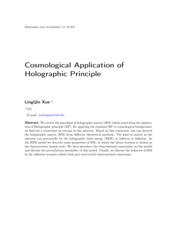
4Holographic Dark Energy4.1HDE in real universeLet’s consider a universe with ordinary matter and holographic matter as holographic darkenergy (HDE), the Friedmann equation can be written as3Mp2 H 2 ρm ρde(4.1)or equivalently:E(z) H(z) H0 Ω0m (1 z)31 Ωde (z) 1/2(4.2)where 2H0ρm0 a0 3 ρcρm Ω0m (1 z)3ρcρc0 aρc0H2ρdeC 2 2 1 ΩmρcL HΩm (4.3)Ωde(4.4)Note that the dark energy energy density is described in Eq.(4.4). Take derivative of ln a: d ln HΩdedΩde 2Ωde 1 (4.5)d ln ad ln aCFrom Eq.(4.1), we obtain:3/23 Ωde Ωded ln H (4.6) d ln a22CCombining two equations we get the dynamical evolution of holographic dark energy: dΩdedΩde2 Ωde (1 z) Ωde (1 Ωde ) 1 (4.7)d ln adzCSince 0 Ωde 1, ddΩlndea is always positive, namely the fraction density of HDE alwaysincreases when the scale factor a(t) increases. This means that the expansion of the universewill never have a turning point, so that the universe will not re-collapse in the future.Solving Eq.(4.7) numerically and substituting the corresponding results into Eq.(4.2), theredshift evolution of Hubble parameter H(z) of the HDE model can be obtained (As examples,see Fig. 8).4.2Equation of StateThe equation of state can be obtained by the continuity equation:dρde 3(1 w)ρde 0d ln a(4.8)Taking the derivative of Eq.(4.1) and combining the result in Eq.(4.6), we obtain the equationof state of HDE: 1 2 Ωdew (4.9)3 3 C– 14 –

Figure 8. The redshift evolution of Hubble parameter H(z) of the HDE model. In this figureΩm0 0.3 is always adopted. The red dotted line, the blue dash-dotted line and the green dashedline correspond to the cases of C 0.6, C 0.8 and C 1, respectively. To make a comparison, wealso plot the result of the ΛCDM model.When the HDE is subdominant Ωde 1, the equation of state w 31 , thus Ωde a 2 .When the HDE is dominants Ωde 1, the equation of state is w 13 23 C, and thus theuniverse experiences accelerating expansion as long as C 0. Such choice of future horizonas the characteristic length yields a component that behaves as dark energy. Moreover, whenC 1, the HDE behaves like cosmological constant Λ. If C 1, the HDE will be similar toa quintessence DE, corresponding to an enternal cosmic expansion; if 0 C 1, the HDEwill behave like phantom DE in the far future corresponding to a cosmic doomsday calledbig rip. This indicates that the parameter C determines the properties of HDE. The value ofC cannot be derived from the theoretical framework of the HDE model, and it can only beobtained by fitting the observational data.4.3Spatial CurvatureIn the conventional picture of ΛCDM inflation, the spatial curvature is very likely tobe negligible. Once inflation lasts much longer than the last 60 e-folds to create the scaleinvaraint power spectrum in CMB, the spatial curvature will be strongly suppressed by theinflation. However, in the framework of HDE predicting 60 e-folds of inflation, the spatialcurvature of our present universe may not be many orders of magnitude less than order one.In [17][18], people take the spatial curvature into account and derive the equation of stateand the expansionthe universe.R ofdt0We use χh t a(t0 ) , and due to the spatial curvature χ Rh . Suppose we still use thefuture horizon as the characteristic lenghth:L a(t)r(χ(t)) a(t)sinn χh– 15 –(4.10)

where we define Ωk 0 k 1 sin xsinn x xΩk 0 k 0 sinh x Ωk 0 k 1Following same steps in Sec.4.1 and Sec.4.2, we can obtain the equation of state: 2p1Ωde cosn χhw 1 3C(4.11)(4.12)where Ωk 0 k 1 cos xcosn x 1Ωk 0 k 0 cosh x Ωk 0 k 1(4.13)and function satisfied that cosn 2 x ksinn 2 x 1. Note that the fraction of spatial curvatureis defined as :C2k(4.14)Ωk 2 2 Ωde 2 2a HH LThus for non-flat universeTherefore1ΩkL2 sinn2 χh22Ωde( k)C a( k)C 2(4.15) 12p2w 1 Ωde C Ωk3C(4.16)qΩdeThis formula also applies to flat universe. Note that there is a constraint that C Ωifk Ωk 0(close) and this is valid for any time. Another bound is given by the second law ofthermal dynamics dS d(πMp2 L2 ) 0:dL 0dtr C Ωde1 Ωk(4.17)Another argument is that the total energy in a region of size L should not exceed the massof a black hole of the same size, 4 3L rs 2GπL ρde C 2 L(4.18)3This will give a bound of parameter C:rΩde C 11 ΩkThe evolution of the HDE is (with radiation into account):"#dΩde12p Ωde (1 Ωde ) Ωde cosn χhd ln aC1 a ΩΩk0de0– 16 –(4.19)(4.20)

Let us consider a universe with a characteristic length scale L. The Holographic Principle tell us that all the physical quantities inside the universe, including the energy density can be described by some quantities on the boundary of the universe. It is clear that only tw