Transcription
Chapter 2Coulomb’s Law2.1 Electric Charge. 2-32.2 Coulomb's Law . 2-3Animation 2.1: Van de Graaff Generator . 2-42.3 Principle of Superposition. 2-5Example 2.1: Three Charges. 2-52.4 Electric Field. 2-7Animation 2.2: Electric Field of Point Charges . 2-82.5 Electric Field Lines . 2-92.6 Force on a Charged Particle in an Electric Field . 2-102.7 Electric Dipole . 2-112.7.1 The Electric Field of a Dipole. 2-12Animation 2.3: Electric Dipole. 2-132.8 Dipole in Electric Field. 2-132.8.1 Potential Energy of an Electric Dipole . 2-142.9 Charge Density. 2-162.9.1 Volume Charge Density. 2-162.9.2 Surface Charge Density . 2-172.9.3 Line Charge Density . 2-172.10 Electric Fields due to Continuous Charge Distributions. 2-18Example 2.2: Electric Field on the Axis of a Rod . 2-18Example 2.3: Electric Field on the Perpendicular Bisector . 2-19Example 2.4: Electric Field on the Axis of a Ring . 2-21Example 2.5: Electric Field Due to a Uniformly Charged Disk . 2-232.11 Summary . 2-252.12 Problem-Solving Strategies . 2-272.13 Solved Problems . 2-292.13.12.13.22.13.32.13.4Hydrogen Atom . 2-29Millikan Oil-Drop Experiment . 2-30Charge Moving Perpendicularly to an Electric Field . 2-31Electric Field of a Dipole. 2-332-1
2.13.5 Electric Field of an Arc. 2-362.13.6 Electric Field Off the Axis of a Finite Rod. 2-372.14 Conceptual Questions . 2-392.15 Additional Problems . .8Three Point Charges. 2-40Three Point Charges. 2-40Four Point Charges . 2-41Semicircular Wire . 2-41Electric Dipole . 2-42Charged Cylindrical Shell and Cylinder . 2-42Two Conducting Balls . 2-43Torque on an Electric Dipole. 2-432-2
Coulomb’s Law2.1 Electric ChargeThere are two types of observed electric charge, which we designate as positive andnegative. The convention was derived from Benjamin Franklin’s experiments. He rubbeda glass rod with silk and called the charges on the glass rod positive. He rubbed sealingwax with fur and called the charge on the sealing wax negative. Like charges repel andopposite charges attract each other. The unit of charge is called the Coulomb (C).The smallest unit of “free” charge known in nature is the charge of an electron or proton,which has a magnitude ofe 1.602 10 19 C(2.1.1)Charge of any ordinary matter is quantized in integral multiples of e. An electron carriesone unit of negative charge, e , while a proton carries one unit of positive charge, e . Ina closed system, the total amount of charge is conserved since charge can neither becreated nor destroyed. A charge can, however, be transferred from one body to another.2.2 Coulomb's LawConsider a system of two point charges, q1 and q2 , separated by a distance r in vacuum.The force exerted by q1 on q2 is given by Coulomb's law:F12 keq1q2rˆr2(2.2.1)where ke is the Coulomb constant, and rˆ r / r is a unit vector directed from q1 to q2 ,as illustrated in Figure 2.2.1(a).(a)(b)Figure 2.2.1 Coulomb interaction between two chargesNote that electric force is a vector which has both magnitude and direction. In SI units,the Coulomb constant ke is given by2-3
ke 14πε 0 8.9875 109 N m 2 / C2(2.2.2)whereε0 1 8.85 10 12 C2 N m 29224π (8.99 10 N m C )(2.2.3)is known as the “permittivity of free space.” Similarly, the force on q1 due to q2 is givenby F21 F12 , as illustrated in Figure 2.2.1(b). This is consistent with Newton's third law.As an example, consider a hydrogen atom in which the proton (nucleus) and the electronare separated by a distance r 5.3 10 11 m . The electrostatic force between the twoparticles is approximately Fe ke e 2 / r 2 8.2 10 8 N . On the other hand, one may showthat the gravitational force is only Fg 3.6 10 47 N . Thus, gravitational effect can beneglected when dealing with electrostatic forces!Animation 2.1: Van de Graaff GeneratorConsider Figure 2.2.2(a) below. The figure illustrates the repulsive force transmittedbetween two objects by their electric fields. The system consists of a charged metalsphere of a van de Graaff generator. This sphere is fixed in space and is not free to move.The other object is a small charged sphere that is free to move (we neglect the force ofgravity on this sphere). According to Coulomb’s law, these two like charges repel eachanother. That is, the small sphere experiences a repulsive force away from the van deGraaff sphere.Figure 2.2.2 (a) Two charges of the same sign that repel one another because of the“stresses” transmitted by electric fields. We use both the “grass seeds” representationand the ”field lines” representation of the electric field of the two charges. (b) Twocharges of opposite sign that attract one another because of the stresses transmitted byelectric fields.The animation depicts the motion of the small sphere and the electric fields in thissituation. Note that to repeat the motion of the small sphere in the animation, we have2-4
the small sphere “bounce off” of a small square fixed in space some distance from thevan de Graaff generator.Before we discuss this animation, consider Figure 2.2.2(b), which shows one frame of amovie of the interaction of two charges with opposite signs. Here the charge on the smallsphere is opposite to that on the van de Graaff sphere. By Coulomb’s law, the two objectsnow attract one another, and the small sphere feels a force attracting it toward the van deGraaff. To repeat the motion of the small sphere in the animation, we have that charge“bounce off” of a square fixed in space near the van de Graaff.The point of these two animations is to underscore the fact that the Coulomb forcebetween the two charges is not “action at a distance.” Rather, the stress is transmitted bydirect “contact” from the van de Graaff to the immediately surrounding space, via theelectric field of the charge on the van de Graaff. That stress is then transmitted from oneelement of space to a neighboring element, in a continuous manner, until it is transmittedto the region of space contiguous to the small sphere, and thus ultimately to the smallsphere itself. Although the two spheres are not in direct contact with one another, theyare in direct contact with a medium or mechanism that exists between them. The forcebetween the small sphere and the van de Graaff is transmitted (at a finite speed) bystresses induced in the intervening space by their presence.Michael Faraday invented field theory; drawing “lines of force” or “field lines” was hisway of representing the fields. He also used his drawings of the lines of force to gaininsight into the stresses that the fields transmit. He was the first to suggest that thesefields, which exist continuously in the space between charged objects, transmit thestresses that result in forces between the objects.2.3 Principle of SuperpositionCoulomb’s law applies to any pair of point charges. When more than two charges arepresent, the net force on any one charge is simply the vector sum of the forces exerted onit by the other charges. For example, if three charges are present, the resultant forceexperienced by q3 due to q1 and q2 will beF3 F13 F23(2.3.1)The superposition principle is illustrated in the example below.Example 2.1: Three ChargesThree charges are arranged as shown in Figure 2.3.1. Find the force on the charge q3assumingthatq1 6.0 10 6 C ,q2 q1 6.0 10 6 C ,q3 3.0 10 6 C anda 2.0 10 2 m .2-5
Figure 2.3.1 A system of three chargesSolution:Using the superposition principle, the force on q3 isF3 F13 F23 q2 q3 1 q1q3 2 rˆ13 2 rˆ23 4πε 0 r13r23 In this case the second term will have a negative coefficient, since q2 is negative. Theunit vectors r̂13 and r̂23 do not point in the same directions. In order to compute this sum,we can express each unit vector in terms of its Cartesian components and add the forcesaccording to the principle of vector addition.From the figure, we see that the unit vector r̂13 which points from q1 to q3 can be writtenas2 ˆ ˆ(i j)rˆ13 cos θ ˆi sin θ ˆj 2Similarly, the unit vector rˆ23 ˆi points from q2 to q3 . Therefore, the total force isq2 q3 1 q1q31 q1q32 ˆ ˆ ( q1 )q3 ˆ (i j) i 2 rˆ13 2 rˆ23 2r23a24πε 0 r13 4πε 0 ( 2a ) 2 1 q1q3 2 ˆ2 ˆ 1ij 4πε 0 a 2 44 F3 upon adding the components. The magnitude of the total force is given by2-6
12221 q1q3 2 2 F3 1 4πε 0 a 2 44 (6.0 10 6 C)(3.0 10 6 C) (9.0 109 N m 2 / C2 )(0.74) 3.0 N(2.0 10 2 m) 2The angle that the force makes with the positive x -axis is F3, y 2/4 1 tan 151.3 1 2 / 4 F3, x φ tan 1 Note there are two solutions to this equation. The second solution φ 28.7 is incorrectbecause it would indicate that the force has positive î and negative ˆj components.For a system of N charges, the net force experienced by the jth particle would beNF j Fij(2.3.2)i 1i jwhere Fij denotes the force between particles i and j . The superposition principleimplies that the net force between any two charges is independent of the presence ofother charges. This is true if the charges are in fixed positions.2.4 Electric FieldThe electrostatic force, like the gravitational force, is a force that acts at a distance, evenwhen the objects are not in contact with one another. To justify such the notion werationalize action at a distance by saying that one charge creates a field which in turn actson the other charge.An electric charge q produces an electric field everywhere. To quantify the strength ofthe field created by that charge, we can measure the force a positive “test charge” q0experiences at some point. The electric field E is defined as:Feq0 0 q0E lim(2.4.1)We take q0 to be infinitesimally small so that the field q0 generates does not disturb the“source charges.” The analogy between the electric field and the gravitational fieldg lim Fm / m0 is depicted in Figure 2.4.1.m0 02-7
Figure 2.4.1 Analogy between the gravitational field g and the electric field E .From the field theory point of view, we say that the charge q creates an electric fieldE which exerts a force Fe q0 E on a test charge q0 .Using the definition of electric field given in Eq. (2.4.1) and the Coulomb’s law, theelectric field at a distance r from a point charge q is given byE qrˆ4πε 0 r 21(2.4.2)Using the superposition principle, the total electric field due to a group of charges isequal to the vector sum of the electric fields of individual charges:E Ei iiqirˆ4πε 0 ri 21(2.4.3)Animation 2.2: Electric Field of Point ChargesFigure 2.4.2 shows one frame of animations of the electric field of a moving positive andnegative point charge, assuming the speed of the charge is small compared to the speed oflight.Figure 2.4.2 The electric fields of (a) a moving positive charge, (b) a moving negativecharge, when the speed of the charge is small compared to the speed of light.2-8
2.5 Electric Field LinesElectric field lines provide a convenient graphical representation of the electric field inspace. The field lines for a positive and a negative charges are shown in Figure 2.5.1.(a)(b)Figure 2.5.1 Field lines for (a) positive and (b) negative charges.Notice that the direction of field lines is radially outward for a positive charge andradially inward for a negative charge. For a pair of charges of equal magnitude butopposite sign (an electric dipole), the field lines are shown in Figure 2.5.2.Figure 2.5.2 Field lines for an electric dipole.The pattern of electric field lines can be obtained by considering the following:(1) Symmetry: For every point above the line joining the two charges there is anequivalent point below it. Therefore, the pattern must be symmetrical about the linejoining the two charges(2) Near field: Very close to a charge, the field due to that charge predominates.Therefore, the lines are radial and spherically symmetric.(3) Far field: Far from the system of charges, the pattern should look like that of a singlepoint charge of value Q i Qi . Thus, the lines should be radially outward, unlessQ 0.(4) Null point: This is a point at which E 0 , and no field lines should pass through it.2-9
The properties of electric field lines may be summarized as follows: The direction of the electric field vector E at a point is tangent to the field lines. The number of lines per unit area through a surface perpendicular to the line isdevised to be proportional to the magnitude of the electric field in a given region. The field lines must begin on positive charges (or at infinity) and then terminate onnegative charges (or at infinity). The number of lines that originate from a positive charge or terminating on a negativecharge must be proportional to the magnitude of the charge. No two field lines can cross each other; otherwise the field would be pointing in twodifferent directions at the same point.2.6 Force on a Charged Particle in an Electric FieldConsider a charge q moving between two parallel plates of opposite charges, as shownin Figure 2.6.1.Figure 2.6.1 Charge moving in a constant electric fieldLet the electric field between the plates be E E y ˆj , with E y 0 . (In Chapter 4, weshall show that the electric field in the region between two infinitely large plates ofopposite charges is uniform.) The charge will experience a downward Coulomb forceFe qE(2.6.1)Note the distinction between the charge q that is experiencing a force and the charges onthe plates that are the sources of the electric field. Even though the charge q is also asource of an electric field, by Newton’s third law, the charge cannot exert a force onitself. Therefore, E is the field that arises from the “source” charges only.According to Newton’s second law, a net force will cause the charge to accelerate with anacceleration2-10
a qEFe qE y ˆjm mm(2.6.2)Suppose the particle is at rest ( v0 0 ) when it is first released from the positive plate.The final speed v of the particle as it strikes the negative plate isvy 2 ay y 2 yqE ym(2.6.3)where y is the distance between the two plates. The kinetic energy of the particle when itstrikes the plate isK 1 2mv y qE y y2(2.6.4)2.7 Electric DipoleAn electric dipole consists of two equal but opposite charges, q and q , separated by adistance 2a , as shown in Figure 2.7.1.Figure 2.7.1 Electric dipoleThe dipole moment vector p which points from q to q (in the y - direction) is givenbyp 2qa ˆj(2.7.1)The magnitude of the electric dipole is p 2qa , where q 0 . For an overall chargeneutral system having N charges, the electric dipole vector p is defined asi Np qi ri(2.7.2)i 12-11
where ri is the position vector of the charge qi . Examples of dipoles include HCL, CO,H2O and other polar molecules. In principle, any molecule in which the centers of thepositive and negative charges do not coincide may be approximated as a dipole. InChapter 5 we shall also show that by applying an external field, an electric dipolemoment may also be induced in an unpolarized molecule.2.7.1 The Electric Field of a DipoleWhat is the electric field due to the electric dipole? Referring to Figure 2.7.1, we see thatthe x-component of the electric field strength at the point P is q cosθ cosθ q xx Ex r 2 4πε 0 x 2 ( y a ) 2 3/ 2 x 2 ( y a) 2 3/ 2 4πε 0 r 2 (2.7.3)wherer 2 r 2 a 2 2ra cos θ x 2 ( y a ) 2(2.7.4)Similarly, the y -component isEy q sin θ sin θ q y ay a (2.7.5) r 2 4πε 0 x 2 ( y a) 2 3/ 2 x 2 ( y a) 2 3/ 2 4πε 0 r 2 In the “point-dipole” limit where rthe above expressions reduce toa , one may verify that (see Solved Problem 2.13.4)Ex 3psin θ cos θ4πε 0 r 3(2.7.6)andEy p4πε 0 r( 3cos θ 1)23(2.7.7)where sin θ x / r and cos θ y / r . With 3 pr cos θ 3p r and some algebra, the electricfield may be written asE( r ) 1 p 3(p r )r 4πε 0 r 3r5 (2.7.8)Note that Eq. (2.7.8) is valid also in three dimensions where r xˆi yˆj zkˆ . Theequation indicates that the electric field E due to a dipole decreases with r as 1/ r 3 ,2-12
unlike the 1/ r 2 behavior for a point charge. This is to be expected since the net charge ofa dipole is zero and therefore must fall off more rapidly than 1/ r 2 at large distance. Theelectric field lines due to a finite electric dipole and a point dipole are shown in Figure2.7.2.Figure 2.7.2 Electric field lines for (a) a finite dipole and (b) a point dipole.Animation 2.3: Electric DipoleFigure 2.7.3 shows an interactive ShockWave simulation of how the dipole pattern arises.At the observation point, we show the electric field due to each charge, which sumvectorially to give the total field. To get a feel for the total electric field, we also show a“grass seeds” representation of the electric field in this case. The observation point can bemoved around in space to see how the resultant field at various points arises from theindividual contributions of the electric field of each charge.Figure 2.7.3 An interactive ShockWave simulation of the electric field of an two equaland opposite charges.2.8 Dipole in Electric FieldWhat happens when we place an electric dipole in a uniform field E E ˆi , with thedipole moment vector p making an angle with the x-axis? From Figure 2.8.1, we seethat the unit vector which points in the direction of p is cos θ ˆi sin θ ˆj . Thus, we havep 2qa(cos θ ˆi sin θ ˆj)(2.8.1)2-13
Figure 2.8.1 Electric dipole placed in a uniform field.As seen from Figure 2.8.1 above, since each charge experiences an equal but oppositeforce due to the field, the net force on the dipole is Fnet F F 0 . Even though the netforce vanishes, the field exerts a torque a toque on the dipole. The torque about themidpoint O of the dipole isτ r F r F (a cos θ ˆi a sin θ ˆj) ( F ˆi ) ( a cos θ ˆi a sin θ ˆj) ( F ˆi ) a sin θ F ( kˆ ) a sin θ F ( kˆ )(2.8.2) 2aF sin θ ( kˆ )where we have used F F F . The direction of the torque is kˆ , or into the page.The effect of the torque τ is to rotate the dipole clockwise so that the dipole momentp becomes aligned with the electric field E . With F qE , the magnitude of the torquecan be rewritten asτ 2a(qE ) sin θ (2aq ) E sin θ pE sin θand the general expression for toque becomesτ p E(2.8.3)Thus, we see that the cross product of the dipole moment with the electric field is equal tothe torque.2.8.1 Potential Energy of an Electric DipoleThe work done by the electric field to rotate the dipole by an angle dθ isdW τ dθ pE sin θ dθ(2.8.4)2-14
The negative sign indicates that the torque opposes any increase in θ . Therefore, the totalamount of work done by the electric field to rotate the dipole from an angle θ 0 to θ isθW ( pE sin θ )dθ pE ( cos θ cos θ 0 )θ0(2.8.5)The result shows that a positive work is done by the field when cos θ cos θ 0 . Thechange in potential energy U of the dipole is the negative of the work done by thefield: U U U 0 W pE ( cos θ cos θ 0 )(2.8.6)where U 0 PE cos θ 0 is the potential energy at a reference point. We shall choose ourreference point to be θ 0 π 2 so that the potential energy is zero there, U 0 0 . Thus, inthe presence of an external field the electric dipole has a potential energyU pE cos θ p E(2.8.7)A system is at a stable equilibrium when its potential energy is a minimum. This takesplace when the dipole p is aligned parallel to E , making U a minimum withU min pE . On the other hand, when p and E are anti-parallel, U max pE is amaximum and the system is unstable.If the dipole is placed in a non-uniform field, there would be a net force on the dipole inaddition to the torque, and the resulting motion would be a combination of linearacceleration and rotation. In Figure 2.8.2, suppose the electric field E at q differs fromthe electric field E at q .Figure 2.8.2 Force on a dipoleAssuming the dipole to be very small, we expand the fields about x : dE dE E ( x a) E ( x) a , E ( x a ) E ( x) a dx dx (2.8.8)The force on the dipole then becomes2-15
dE ˆFe q (E E ) 2qa i dx dE p î dx (2.8.9)An example of a net force acting on a dipole is the attraction between small pieces ofpaper and a comb, which has been charged by rubbing against hair. The paper hasinduced dipole moments (to be discussed in depth in Chapter 5) while the field on thecomb is non-uniform due to its irregular shape (Figure 2.8.3).Figure 2.8.3 Electrostatic attraction between a piece of paper and a comb2.9 Charge DensityThe electric field due to a small number of charged particles can readily be computedusing the superposition principle. But what happens if we have a very large number ofcharges distributed in some region in space? Let’s consider the system shown in Figure2.9.1:Figure 2.9.1 Electric field due to a small charge element qi .2.9.1 Volume Charge DensitySuppose we wish to find the electric field at some point P . Let’s consider a smallvolume element Vi which contains an amount of charge qi . The distances betweencharges within the volume element Vi are much smaller than compared to r, thedistance between Vi and P . In the limit where Vi becomes infinitesimally small, wemay define a volume charge density ρ (r ) as qi dq Vi 0 VdViρ (r ) lim(2.9.1)2-16
The dimension of ρ (r ) is charge/unit volume (C/m3 ) in SI units. The total amount ofcharge within the entire volume V isQ qi ρ (r ) dVi(2.9.2)VThe concept of charge density here is analogous to mass density ρ m (r ) . When a largenumber of atoms are tightly packed within a volume, we can also take the continuumlimit and the mass of an object is given byM ρ m (r ) dV(2.9.3)V2.9.2 Surface Charge DensityIn a similar manner, the charge can be distributed over a surface S of area A with asurface charge density σ (lowercase Greek letter sigma):σ (r ) dqdA(2.9.4)The dimension of σ is charge/unit area (C/m 2 ) in SI units. The total charge on the entiresurface is:Q σ (r ) dA(2.9.5)S2.9.3 Line Charge DensityIf the charge is distributed over a line of length(lowercase Greek letter lambda) is λ (r ) dqd, then the linear charge density λ(2.9.6)where the dimension of λ is charge/unit length (C/m) . The total charge is now anintegral over the entire length:Q λ (r ) d(2.9.7)line2-17
If charges are uniformly distributed throughout the region, the densities ( ρ , σ or λ ) thenbecome uniform.2.10 Electric Fields due to Continuous Charge DistributionsThe electric field at a point P due to each charge element dq is given by Coulomb’s law:dE 1 dqrˆ4πε 0 r 2(2.10.1)where r is the distance from dq to P and r̂ is the corresponding unit vector. (See Figure2.9.1). Using the superposition principle, the total electric field E is the vector sum(integral) of all these infinitesimal contributions:E 1dq r4πε 0 V2rˆ(2.10.2)This is an example of a vector integral which consists of three separate integrations, onefor each component of the electric field.Example 2.2: Electric Field on the Axis of a RodA non-conducting rod of length with a uniform positive charge density λ and a totalcharge Q is lying along the x -axis, as illustrated in Figure 2.10.1.Figure 2.10.1 Electric field of a wire along the axis of the wireCalculate the electric field at a point P located along the axis of the rod and a distance x0from one end.Solution:The linear charge density is uniform and is given by λ Q / . The amount of chargecontained in a small segment of length dx ′ is dq λ dx′ .2-18
Since the source carries a positive charge Q, the field at P points in the negative xdirection, and the unit vector that points from the source to P is rˆ ˆi . The contributionto the electric field due to dq isdE 1 dq1 λ dx′ ˆ1 Qdx′ ˆrˆ i( i ) 224πε 0 r4πε 0 x′4πε 0 x′2Integrating over the entire length leads toE dE 1 Q4πε 0 x0 x0dx′ ˆ1 Q 11 ˆ1Qˆi (2.10.3)i i 24πε 0 x0 x0 4πε 0 x0 ( x0 )x′Notice that when P is very far away from the rod, x0becomesE , and the above expression1Qˆi4πε 0 x02(2.10.4)The result is to be expected since at sufficiently far distance away, the distinctionbetween a continuous charge distribution and a point charge diminishes.Example 2.3: Electric Field on the Perpendicular BisectorA non-conducting rod of length with a uniform charge density λ and a total charge Qis lying along the x -axis, as illustrated in Figure 2.10.2. Compute the electric field at apoint P, located at a distance y from the center of the rod along its perpendicular bisector.Figure 2.10.2Solution:We follow a similar procedure as that outlined in Example 2.2. The contribution to theelectric field from a small length element dx ′ carrying charge dq λ dx′ is2-19
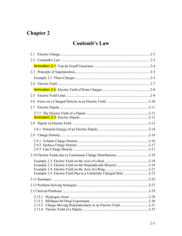
dE dq1λ dx′ 24πε 0 r ′4πε 0 x′2 y 21(2.10.5)Using symmetry argument illustrated in Figure 2.10.3, one may show that the x component of the electric field vanishes.Figure 2.10.3 Symmetry argument showing that Ex 0 .The y-component of dE isdE y dE cos θ λ dx′14πε 0 x′ y2y2x ′2 y 2 1λ y dx′4πε 0 ( x′ y 2 )3/ 22(2.10.6)By integrating over the entire length, the total electric field due to the rod isE y dE y 14πε 0 /2 /2λ ydx′( x′ y )22 3/ 2 λy4πε 0 dx′/ 2 ( x′ y 2 )3/ 2/2 2(2.10.7)By making the change of variable: x′ y tan θ ′ , which gives dx′ y sec 2 θ ′ dθ ′ , theabove integral becomes θdx′y sec2 θ ′dθ ′1 θ sec 2 θ ′dθ ′1 2223/2323/2223/2 θ y (sec θ ′ 1)/ 2 ( x′ y )y θ (tan θ ′ 1)y1 θ dθ ′1 θ2sin θ 2 2 cos θ ′dθ ′ θθ ysec θ ′ yy2/2sec2 θ ′dθ ′ θ secθ ′3θ(2.10.8)which givesEy 2λ sin θ1 2λ 4πε 04πε 0 yy1/2y ( / 2) 22(2.10.9)2-20
In the limit where y, the above expression reduces to the “point-charge” limit:Ey On the other hand, when2λ / 21 λ1 Q 24πε 0 y y4πε 0 y4πε 0 y 21(2.10.10)y , we haveEy 2λ4πε 0 y1(2.10.11)In this infinite length limit, the system has cylindrical symmetry. In this case, analternative approach based on Gauss’s law can be used to obtain Eq. (2.10.11), as weshall show in Chapter 4. The characteristic behavior of E y / E0 (with E0 Q / 4πε 0 2 ) asa function of y /is shown in Figure 2.10.4.Figure 2.10.4 Electric field of a non-conducting rod as a function of y / .Example 2.4: Electric Field on the Axis of a RingA non-conducting ring of radius R with a uniform charge density λ and a total charge Qis lying in the xy - plane, as shown in Figure 2.10.5. Compute the electric field at a pointP, located at a distance z from the center of the ring along its axis of symmetry.Figure 2.10.5 Electric field at P due to the charge element dq .2-21
Solution:Consider a small length element d ′ on the ring. The amount of charge contained withinthis element is dq λ d ′ λ R dφ ′ . Its contribution to the electric fiel
The smallest unit of “free” charge known in nature is the charge of an electron or proton, which has a magnitude of e 1.602 10 19 C (2.1.1) Charge of any ordinary matter is quantized in integral multiples of e. An electron carries one unit of negative charge, e, w