Transcription
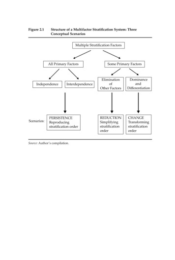
36Color Lines, Country LinesFigure 2.1Structure of a Multifactor Stratification System: ThreeConceptual ScenariosMultiple Stratification FactorsAll Primary TENCEReproducingstratification orderSome Primary FactorsEliminationofOther ationorderSource: Author’s compilation.Should nativity then be eliminated as a stratification factor? I propose afurther distinction between elimination, in which a secondary factor (nativity) is eliminated because it does not differentiate within groups, anda two-tiered system of dominance-differentiation, in which primary factors (race and class) dominate and secondary factors (nativity) differentiate within groups. The elimination of a factor reduces the complexity ofsocial inequality and simplifies the stratification order—a scenario of reduction. On the other hand, the dominance-differentiation system provides an opportunity for change in an unusual way. Although primaryfactors dominate initially, differentiation by secondary factors withinprimary-factor groups creates great within-group variations, ultimatelyleading to the weakening of the divides by the primary factors. For instance, concerning wealth, Hong Kong and Taiwan immigrants surpassnative whites, Cuban immigrants within the Hispanic group are comparable with the Asian group and Dominican immigrants within the Hispanic group are comparable with the black group. These differentiations
Wealth Distribution, An OverviewFigure 3.1Wealth Holding Status by Race-EthnicitySufficientInsufficientAsset poorNet 20.10WhiteBlackHispanicAsianSource: Author’s compilation.Figure 3.20.6Wealth Holding Status by Education LevelsSufficientInsufficientAsset poorNet 10Bachelor’sSource: Author’s compilation.Some collegeH.S. H.S.57
58Color Lines, Country LinesFigure 3.3Wealth Holding Status by NativitySufficientInsufficientAsset poor0.6Net 10NativeImmigrantSource: Author’s compilation.Figure 3.40.6Wealth Holding Status by Age GroupSufficientInsufficientAsset poorNet 1025 to 34Source: Author’s compilation.35 to 4445 to 5455 to 64
Wealth Distribution, An OverviewFigure 3.5Net Worth Percentile Distribution by Race-EthnicityWhiteHispanic110Net Worth in 1000061BlackAsian805020 100.1.2.3.4.5p.6.7.8.91Source: Author’s compilation.Figure 3.6Net Worth Percentile Distribution by Education LevelsBachelor’sHigh SchoolSome College High SchoolNet Worth in 10000110805020 100.1.2Source: Author’s compilation.3.4.5p.6.7.8.91
62Color Lines, Country LinesFigure 3.7Net Worth Percentile Distribution by NativityNet Worth in 10000110NativeImmigrant805020 100.1.2.3.4.5p.6.7.8.91.91Source: Author’s compilation.Figure 3.8Net Worth Percentile Distribution by Age Group25 to 3445 to 5435 to 4455 to 64Net Worth in 10000110805020 100.1.2Source: Author’s compilation.3.4.5p.6.7.8
Wealth Distribution, An OverviewFigure 3.967Age Profiles of Net Worth by Race-Ethnicity140WhiteBlackHispanicAsianNet Worth in 10001201008060402002530354045Age50556065Source: Author’s compilation.Figure 3.10Age Profiles of Net Worth, Nativity–Within White180NativeImmigrantNet Worth in 100015012090603002530Source: Author’s compilation.354045Age50556065
68Color Lines, Country LinesFigure 3.11Age Profiles of Net Worth, Nativity–Within Black180NativeImmigrantNet Worth in 100015012090603002530354045Age50556065Source: Author’s compilation.Figure 3.12Age Profiles of Net Worth, Nativity–Within Hispanic180NativeImmigrantNet Worth in 100015012090603002530Source: Author’s compilation.354045Age50556065
Wealth Distribution, An OverviewFigure 3.1369Age Profiles of Net Worth, Nativity–Within Asian180NativeImmigrantNet Worth in 100015012090603002530354045Age50556065Source: Author’s compilation.low the entire life cycles of birth and arrival cohorts to tease out the age,period, and cohort effects. Existing data, such as censuses and surveys,do not follow households for the entire life cycle, and thus are not ideal.Such data limitation raises a double challenge to ascertaining nativitydifferences in life cycle wealth patterns: a need to separate both age, period, and cohort effects for all households and the effects of length of residence and arrival cohorts for immigrant households. The first challengecomes in the perfect linear combination of age (of a householder), period(of a calendar year), and birth cohort (of a group of householders born inthe same year) as age equals calendar year minus birth year, a wellknown dilemma in population studies (Ryder 1964; Mason and Fienberg1985). By the same token, the second challenge comes in the perfect linear combination of length of residence, calendar year, and arrival cohort(a group of immigrants arriving in the United States in the same year) aslength of residence equals calendar year minus arrival year (Myers andLee 1996).When only one cross-section of data is available, researchers use asynthetic cohort, which is based on data from several age cohorts andshows hypothetical observations over time. For instance, if on average
72Color Lines, Country LinesFigure 3.14Net Worth in 100011080Age Profile of Net Worth, Synthetic Cohorts in 1996NativeArrival 1965 to 1974Arrival 1975 to 1984Arrival post-19845020 1025 27 29 31 33 35 37 39 41 43 45 47 49 51 53 55 57 59 61 63 65AgeSource: Author’s compilation.arrival cohorts in 1996: later ages for the earlier and earlier ages for thelater arrival cohort. Relative to natives’ wealth profile, the 1965 to 1974cohort is moderately worse off, the 1975 to 1984 cohort’s wealth profilestarted to rise at age thirty-seven but fell at age forty-seven, and the post1984 cohort’s wealth profile is notably low and flat. That these four profiles do not connect challenges the synthetic cohort assumption that latercohorts would follow the track of earlier cohorts.Synthetic Cohort with Pooled Cross-SectionsThe major advantage of a synthetic cohort with pooled cross-sectionsover a synthetic cohort with one cross-section is the allowance for fullerobservations of immigrant arrival cohorts (see the complete profiles forthe four arrival cohorts in figure 3.15). Figure 3.15 uses eighteen crosssections from the years from 1984 to 2003. We see that at age thirty-nine,the 1965 to 1974 arrival cohort falls below the native profile. The 1975 to1984 cohort members’ wealth stops growing after age forty-five, and thepost-1984 cohort’s wealth profile remains flat at all ages. Other than dataimprovements, the patterns shown in figure 3.15 resemble those in figure
Wealth Distribution, An OverviewFigure 3.15Age Profile of Net Worth, Synthetic Cohorts 1984 to 2003110Net Worth in 100073NativeArrival 1965 to 1974Arrival 1975 to 1984Arrival post-1984805020 1025 27 29 31 33 35 37 39 41 43 45 47 49 51 53 55 57 59 61 63 65AgeSource: Author’s compilation.3.14 and may be contaminated by the unsubstantiated assumptions ofsynthetic cohort approach.Cohort EvolutionA cohort evolution approach takes advantage of the eighteen cross-sections to depict birth cohort evolution along the life cycle and to check thebirth cohort assumption of the synthetic cohort approach. Here, thatlater birth cohorts will trace the same trajectory of earlier birth cohorts isno long assumed. Instead, separate profiles are drawn for natives andimmigrants for each of the six cohorts. Because the data cover only twodecades but the age range is forty years, we can follow birth cohort evolution for shorter periods for the oldest and youngest cohorts and longerperiods for those in the middle. Figures 3.16 and 3.17 are for natives andimmigrants, respectively. In figure 3.16, the six age profiles connectnicely to form an underlying native profile very similar to the one in figure 3.15. This suggests that the synthetic cohort assumption holds for natives. The synthetic cohort approach may therefore be appropriate forthe native population. Figure 3.17, however, does not suggest the same
74Color Lines, Country LinesFigure 3.16Age Profile of Net Worth, Evolution of Native Birth Cohorts,1984 to 2003140Born 1920 to 1929Born 1930 to 1939Born 1940 to 1949Born 1950 to 1959Born 1960 to 1969Born 1970 to 1979Net Worth in 1000120100806040200253035404550Cohort Median Age556065Source: Author’s compilation.Figure 3.17Age Profile of Net Worth, Evolution of Immigrant BirthCohorts, 1984 to 2003140Born 1920 to 1929Born 1930 to 1939Born 1940 to 1949Born 1950 to 1959Born 1960 to 1969Born 1970 to 1979Net Worth in 10001201008060402002530Source: Author’s compilation.35404550Cohort Median Age556065
76Color Lines, Country LinesFigure 3.18Age Profile of Net Worth, Evolution of 1950 to 1959 BirthCohort, 1984 to 2003Net Worth in 100080NativeArrival 1965 to 1974Arrival 1975 to 1984604020030323436384042Cohort Median Age444648Source: Author’s compilation.Figure 3.19Age Profile of Net Worth, Evolution of 1960 to 1969 BirthCohort, 1984 to 2003Net Worth in 100040NativeArrival 1965 to 1974Arrival 1975 to 1984Arrival after 198430201002527Source: Author’s compilation.293133Cohort Median Age353739
Wealth Distribution, An OverviewFigure 3.20Age Profile of Net Worth, Evolution of 1970 to 1979 BirthCohort, 1984 to 200310NativeArrival 1965 to 1974Arrival 1975 to 1984Arrival 1985 to 20038Net Worth in 100077642025262728Cohort Median Age2930Source: Author’s compilation.at a lower point than the native born, but the two earlier arrival cohortsspeed up and the most recent cohort fails to do so. Taken together, thethree birth cohorts depicted in figures 3.18 through 3.20, both native andimmigrant, appear to fare successively worse. For instance, at age thirty,the median net worth is lower for those born later than for those bornearlier. This may reflect a period effect.The major lesson we have learned from these examinations is thatportraying life cycle patterns of wealth for immigrants requires extremecare. Although the synthetic cohort approach is appropriate for natives,it yields misleading results for immigrants. The method here, followingcohort evolution and keeping PAYUS constant, provides more appropriate comparisons than the traditional synthetic cohort or cohort evolutionapproaches, which do not consider PAYUS.ConclusionThe national picture of wealth disparity, then, can be described both qualitatively and quantitatively. The qualitative measure includes five categories of wealth holding status—sufficient, insufficient, and asset-pooramong those with positive net worth, and net debtor and paycheck-to-
Wealth Distribution, An OverviewTable 3.159Percentage Distribution of Wealth Holding Status by Nativity andDemographic Characteristics, in torPaycheckto-Paycheck% nBachelor’sSome collegeHigh schoolSchooling .23.52.93.125.130.825.918.2GroupSource: Author’s compilation.Note: The statistics are the average for the years 1984 to 2003.The data are based on respondents whose net worth is within the lower 99.5 percent of the originalnet worth distribution in the SIPP data (see appendix for details).groups or among education groups.Wealth is accumulated along the life cycle of a household, captured bythe householder’s age. Figure 3.4 shows the pattern of wealth holdingstatus by four age groups. The life cycle pattern is clearly seen from themonotonic increase of being sufficient and decline in all other statuses.In examining wealth holding statuses by the four basic demographiccharacteristics, we have learned about the stratification of wealth, whichis measured qualitatively. The refined definition of wealth holding basedon the asset poverty concept helps reveal the stratification by race-ethnicity, education, nativity, and age. It is essential to distinguish the bestoff (sufficient) and worst off (paycheck-to-paycheck) among various demographic groups. The stratification by race-ethnicity, education levels,and age groups are much wider than that by nativity. These qualitativemeasures, however, cannot reflect the levels and variations of wealthamong demographic groups. We now turn to these issues.
Table 3.2GroupSelected Percentiles of Net Worth, Asset, and Debt by Race-Ethnicity (2001 Dollars)5th10th25th50th75th90th95th99thNet WorthTotalWhiteBlackHispanicAsian 8,850 8,023 11,111 10,982 11,130 975 90 3,347 3,125 00405,700422,969261,865322,156517,622Source: Author’s compilation.Note: The statistics are the average for the years 1984 to 2003.Percentiles are based on respondents whose net worth is within the lower 99.5 percent of the original net worth distribution in the SIPP data.
Table 3.3PercentileSelected Percentiles of Net Worth, Asset, and Debt: by Nativity (2001 Dollars)5th10th25th50th75th90th95th99thNet WorthNativeImmigrant 8,772 9,416 886 4Source: Author’s compilation using data from the SIPP 1984 2001 panels.Note: The statistics are the average for the years 1984 to 2003.Percentiles are based on respondents whose net worth is within the lower 99.5 percent of the original net worth distribution in the SIPP data.
Latino ImmigrantsFigure 4.181Demographics by Latino Group0.8Proportion0.60.40.20.0nv wht nv hsp25 to 44COLmarriededucation 12SLVGMNno childrenMEXCUBDOM3 children 1.3 poverty rateSource: Author’s compilation.constant U.S. dollars) in 2003 (World Bank 2005), placing the country inthe middle to lower tier of Latin America’s economic development. Recent and rapid urbanization has led to an urban population of about 75percent of the population. Although the government mandates nineyears of education, only five years are offered in rural areas (World Bank2005). A former Spanish colony, Colombia gained its independence in1819 (Sturges-Vera 1990). Recent decades have witnessed civil wars, insurgent movements, and guerrilla warfare. No single explanation fullyaddresses the deep roots of the troubles Colombia sees today, but amongthe contributing factors are social inequities, lack of state presence in rural areas, the expansion of illicit drug cultivation, and the violence thataccompanies it.Figure 4.1 shows that almost 60 percent of Colombian immigranthouseholds are younger, a higher percentage than native whites but alower one than Latino Americans, indicating that Colombians have relatively slow chain migration. The marriage rate for Colombians is lowerthan for native whites and higher than for Latino Americans. This maybe in part due to the relatively younger age structure. The proportionhaving three or more children (5 percent) is also surprisingly low, even
Latino ImmigrantsFigure 4.289Wealth Holding Status by Latino Group1009080Percentage706050403020100nv wht nv hspCOLSLVGMNMEXCUBDOMSufficientInsufficientAsset poorNet debtorPaycheck-to-paycheckSource: Author’s compilation.top group among all Latinos, whether natives or immigrants, almostreaching parity with native whites. A hidden difference, however, lies inthe relatively lower consumption levels of Cuban immigrants ( 44,000)when compared to native whites ( 53,000). Nonetheless, Cubans surpassnative Latinos by a wide margin. It appears that nativity differences aretrivial in comparison with differences by origin countries. This point isfurther supported by examining other Latino immigrant groups.Economic security is hard to achieve among Latino immigrant groupsother than Cubans. The least secure group is Dominican, with only 15percent having sufficient wealth and only about 30 percent living abovethe asset poverty line (total net worth equals three months living expenses at the official poverty line). Colombian, Salvadoran, Guatemalan,and Mexican immigrants are better off than Dominicans but worse offthan native Latinos and Cubans. These patterns suggest that when economic buffers are concerned, differences in nativity are smaller thanthose among Latino immigrant groups.With an important modification of the notion that Robert Havemanand Edward Wolff first introduced (2004), asset poverty defined in thisvolume is the financial situation when a household owns less positivenet worth than what is needed to maintain the household at the poverty
Latino ImmigrantsFigure 4.393Percentile Distribution of Net Worth by Latino GroupNet Worth in 10000140110805020 100.1.2.3.4.5.6.7.8.91pNative whiteColombianGuatemalanCubanNative HispanicSalvadoranMexicanDominicanSource: Author’s compilation.cause the distributions of net worth, assets, and debts are widely spreadand highly skewed, examining the distribution—rather than the mean ormedian—is more productive. To depict the distributions’ unevenness,we first draw the percentile distribution of net worth for native whites,native Latinos, and the six Latino immigrant groups in figure 4.3. Wethen report three exact percentiles in the distribution—the fifth, fiftieth,and ninety-fifth percentiles—for details.Figure 4.3 draws the 99 percentiles of net worth against the cumulative proportion of the population, for each of the groups in comparison.Because net worth is highly right-skewed, we see a relatively flat curvefor the lower 70 percent of the population. The higher the position of thecurve for a group, the higher the level of net worth. Native whites havethe highest net worth except in the bottom 30 percent of the distribution.The Cuban curve is located not much below the native white curve, andall other group curves, including the native Latino, lie much lower thanthe native white. The Dominican curve is the lowest.The left panel of table 4.3 shows the three selected percentiles of networth. The median for native whites is about 72,000, more than fourtimes that for Latino Americans ( 16,000) and about twice that for
96Color Lines, Country LinesFigure 4.4Net Worth and Debts as Percentage of Native White Assets byLatino Group100Percentage806040200nv wht nv hspNet worthCOLSLVSecured debtGMNMEXUnsecured debtCUBDOMgapSource: Author’s compilation.may reduce future assets. I express net worth, secured debt, and unsecured debt each as a percentage of two bases—native whites’ average total assets (see figure 4.4) and the group-specific total assets (see figure4.5). Figure 4.4 facilitates between-group comparisons and figure 4.5 facilitates within-group analysis.In figure 4.4, the three sections of the bar for native whites denote networth, unsecured debt, and secured debt as a percentage of the total assets. For other groups, in addition to the sections for net worth, secureddebt, and unsecured debt each as a percentage of native whites’ total assets, the top section denotes the gap in total assets between the groupand native whites. For instance, the gap between native whites andLatino Americans is nearly 50 percent, meaning that the total assets ofthe average Latino American household are about 50 percent those of theaverage native white household. Comparing a particular section (for example, secured debts) across bars reveals the absolute size differencesacross groups. For instance, Cubans have a lower level of net worth thannative whites but both groups carry similar secured debt.The graph shows lower absolute amounts of net worth for all Latinogroups than for native whites and yet a wide variation among Latinogroups. Compared with the large net worth variation, the secured debtvariation is smaller. A key institutional factor in asset building is thelending market. Before 1995, when home equity loans did not yet allow
98Color Lines, Country LinesFigure 4.5Net Worth and Debt as Percentage of Total Assets by Latino Group100Percentage806040200nv wht nv hspNet worthCOLSLVSecured debtGMNMEXCUBDOMUnsecured debtSource: Author’s compilation.Unsecured debts include consumer debt, medical bills, private debt, andloans from banks that are not for asset building. Guatemalan immigrantshave the largest unsecured debt share among the groups shown in figure4.5. However, given the low value of their total assets, their large unsecured debt share should not be taken as a sign of huge consumer debts.This portfolio examination indicates that even Latino immigrant groupswho are better off do not have an immediate financial buffer and thus arenot in a mature asset building stage. Those who are worse off have assetvalues too low for any meaningful discussion of future financial buffers.Theoretically, a household can liquidate all its assets, pay off all its secured debt, and use the balance to cover living costs in an emergency situation. Total equity is used to mean the balance between total assets andtotal secured debt. Realistically, homes and retirement accounts are lessliquid than other equity, such as bank accounts, stocks and bonds, andother real estate. I call home and retirement accounts quasi-liquid andthe other seven components liquid. Figure 4.6 describes nine portfoliocomponents as percentages of the specific group’s total equity. Each barconsists of nine sections: home equity (home); IRA, Keogh, and 401(k)accounts (ira); interest-earning saving and checking accounts, money
Latino ImmigrantsFigure 4.699Portfolio as Percentage of Total Equity by Latino Group100Percentage806040200nv wht nv OMvehclSource: Author’s compilation.market deposit accounts, and certificates of deposit (intbk); municipalbonds, corporate bonds and U.S. securities (intot); non–interest earningchecking accounts, saving bonds, and other financial investment (otast);sale value of cars (vehcl); business equity (beq); stocks and mutual funds(stk); other real estate (ore). If the group’s total equity is adequate, asmaller percentage of home equity indicates a higher capacity and preference for diverse financial investments. Native whites’ home equity isabout 40 percent of their total. The proportion for Latino Americans,Colombian immigrants, and Cuban immigrants is about 50 percent, alsoindicating diverse investment behavior. By contrast, given their low levels of equity, Mexican, Salvadoran, Guatemalan, and Dominican immigrants can invest only in their homes. Retirement accounts weigh moreheavily for native whites than for any other group, but Latino Americans, Colombian immigrants, and Cuban immigrants also gravitate toward retirement savings. As might be expected, other Latino immigrantgroups, who have a higher propensity for return migration, show a lowpreference for saving for old-age security, at least in the United States.Business equity, though included here as a component, is fundamen-
Latino ImmigrantsFigure 4.7105Crude and Adjusted Homeownership Rates by Latino Group0.8Rate0.60.40.20.0nv wht nv hspCOLcrudeSLVadj1GMNadj3MEXCUBDOMadj4Source: Author’s compilation.homeownership. This suggests that, rather than female headship, human capital is the key to elevate this group out of poverty and welfaredependency.As a whole, the patterns emerging from table 4.4 and figure 4.7 suggest that the compositions of age, marital status, and number of childrendo not help explain much of the white-Latino homeownership gaps.However, education composition does explain a substantial portion. Wenow turn to investigate whether each demographic characteristic affectshomeownership differently within groups.Differential EffectsThe age effect captures income growth and motives to save along the lifecycle. The marriage effect may differ among groups because somegroups may not have the asset building advantage that married nativewhite households have. A lower return on human capital for racial minorities and those holding foreign degrees, residential segregation byrace or class, more responsibility for extended families, weaker saving
Latino ImmigrantsFigure 4.8109Crude and Adjusted Negative Home Equity Rates AmongHomeowners, by Latino Group0.12Rate0.080.040.00nv wht nv hspCOLcrudeSLVadj1GMNadj3MEXCUBDOMadj4Source: Author’s compilation.marriage and children do not have much influence on Latino immigranthomeownership. When the compositions of demographic characteristicsare held constant, homeownership rates are similar between Cuban immigrants and native whites but lower for other Latino immigrantTable 4.6Negative Home Equity Rates Among Homeowners byLatino GroupCrudeAdj1aAdj3bAdj4cNative whiteLatino 0090.0620.0230.026Source: Author’s compilation.a Adj1 adjusts for age composition.b Adj3 adjusts for the composition of age, marital status, and number of children.c Adj4 adjusts for the composition of age, marital status, number of children, and education levels.
116Color Lines, Country LinesFigure 4.9Financial Asset Rates by Latino .070.00nv wht nv hspstkint-bankCOLSLVcheckingGMNMEXliquid crudeCUBDOMliquid adjSource: Author’s compilation.household pool 20,000 from their liquid financial assets to pay for theiressential needs? The last two bars for each group present the crude rateof owning liquid assets of at least 20,000 and the corresponding rate adjusted for the composition of age, marital status, number of children, andeducation levels. Native whites (the baseline group) are the most likelyto have at least 20,000 in liquid assets (28.4 percent). The crude rates forall other groups are much lower. Cuban immigrants rank a distant second at 17.4 percent but higher than Latino Americans at 12.7 percent. Therates for other immigrant groups are very low, particularly Salvadorans,Guatemalans, Mexicans, and Dominicans, all lower than 6 percent. Afteradjusting for demographic composition, all nonwhite groups improve,with Dominican immigrants seeing the greatest increase (from 3.7 to 14.3percent).Overall, all Latino immigrant groups seem to lag behind native whitesin their rates of investing in the modern financial economy in the forms ofstocks and mutual funds. Perhaps the most striking finding is that Latinoimmigrant households have much lower levels of liquid financial assetseven when their demographic compositions are comparable to those ofnative whites. This makes Latino households financially vulnerable.
118Color Lines, Country LinesFigure 4.10Crude and Adjusted Retirement Account Rates by Latino Group0.60Rate0.400.200.00nv wht nv hspira crudeCOLSLVGMNMEXira adj401k crudetotal crudetotal adjCUBDOM401k adjSource: Author’s compilation.neither IRAs nor Keoghs include employer contributions. I maintain401(k) accounts separately because they often include employer contribution. Households in which the head is older than fifty-nine or households with liquid assets in excess of 20,000 are more likely to own retirement accounts (Gale and Scholz 1994). The early withdrawal penaltydiscourages young households or households with limited liquid financial assets from setting up retirement accounts because of the high transaction costs when early withdrawal is likely. Thus, a more valid groupcomparison must adjust for the composition of these two characteristics.Figure 4.10 shows both the crude rates and the rates adjusted for thecomposition of head of household’s age (younger or older than fifty) andhousehold’s liquid financial assets (less or more than 20,000).Among native whites, the crude rate of IRA-Keogh ownership is 30.8percent, much higher than any other group. The Cuban immigrant rateis 16.8 percent, which though a low second is far above the remaininggroups. At the bottom are Guatemalan, Salvadoran, Mexican, and Dominican immigrants, with rates ranging from 0 to 3 percent. Adjustingfor the composition of age and liquid financial asset compositions leadsto a large increase in the adjusted rates for Latino Americans, Colombian,Mexican, Cuban, and Dominican immigrant groups and virtually nochange for Salvadoran immigrants.4
Latino ImmigrantsFigure 4.11121Crude and Adjusted Life Insurance Rates by Latino v wht nv hspemp crudeCOLSLVemp adjtotal crudeGMNMEXself crudetotal adjCUBDOMself adjSource: Author’s compilation.likely to be insured. Adjusting for the demographic compositions of native whites narrows the life insurance gap somewhat, but it still remainslarge. The overall low rates of life insurance ownership among Latinoimmigrants reflect that some of them plan an eventual return to theircountries and therefore feel no need to purchase this type of insurance inthe United States.Table 4.12Life Insurance by Latino GroupEmployer-ProvidedSel
Some College High School Figure 3.6 Net Worth Percentile Distribution by Education Levels Source: Author’s compilation. 62 Color Lines, Country Lines Net Worth in 10000 110 80 50 20 . (of a calendar year), and birth cohort (of a group of householders born in the same year) as age equals