Transcription
Chapter 1ADAMS/Solver and MSSIntroductionThis “Overview” introduces the computer program Automatic Dynamic Analysis ofMechanical Systems (ADAMS). Engineers use ADAMS/Solver in the field ofMechanical System Simulation (MSS) to simulate both large and small scale motion ofmechanical systems. These motions are induced by the action of applied forces orexcitations that act upon the system.The purpose of this Overview is to help you use ADAMS/Solver to design and analyzemechanical systems from the most elementary pendulum, or four-bar mechanism, tothe very complex suspension systems and other sophisticated mechanical devices. Ifyou are a more experienced ADAMS/Solver user, you will learn about the most recentinnovations in the code.This Overview includes the following chapters and appendix:1.ADAMS/Solver and MSS. Describes the role of ADAMS/Solver simulationcode in the field of Mechanical Systems Simulation.2.Modeling Concepts. Introduces necessary ideas to construct models for anADAMS/Solver analysis.3.Modeling Process. Describes a sequence of steps to create an ADAMS/Solvermodel, run a simulation, and review the results.4.ADAMS/Solver Statements. Defines the syntax and format of statements usedto define input for an ADAMS/Solver simulation.5.Customizing ADAMS/Solver. Describes customizing procedures to definenonstandard modeling elements or to generate nonstandard output.6.Executing ADAMS/Solver. Discusses procedures to initiate anADAMS/Solver simulation and to control the process.7.Output Files. Summarizes the purpose and contents of various output files.Appendix A. “The Ten Easy Steps to Happy Simulations.” Methods for avoidingthe commonly encountered pitfalls associated with ADAMS/Solver models.An Overview of How to Use ADAMS/Solver1
Chapter 1. ADAMS/Solver and MSS1.1 Definition of MSSMechanical System Simulation (MSS) is the study of the motion of mechanicalsystems caused by external forces and excitations that act on the system. MSSsimulates large displacement motion, i.e., the extent of the relative motion of thecomponents can be on the order of the overall dimensions of the system. Themechanical system consists of rigid and flexible parts interconnected by various kindsof joints and other constraining forces. The net reaction and applied forces drive therelative motion of the parts.MSS software is of growing, fundamental importance to modern MechanicalComputer-Aided Engineering (MCAE). It allows you to evaluate the designcharacteristics and performance of a product prior to fabrication of the prototype. WithMSS software, you can reduce product development costs, evaluate more designalternatives, and reduce the time it takes to bring a new product to market.2An Overview of How to Use ADAMS/Solver
Chapter 1. ADAMS/Solver and MSS1.2 The Relationship of MSS to Other TechnologiesThe MSS software complements other programs used for Mechanical Computer-AidedEngineering. MSS can incorporate data from other software products into a completesimulation of system behavior. MSS also produces output that assists in furtheranalysis with other computational tools.As Figure 1 illustrates, MSS software exchanges data with other applications. Adiscussion of these applications follows Figure signComponentActuationModelingModalAnalysisFigure 1. MSS Software1.Computer-Aided Design (CAD) creates mechanical models for MSS anddisplays MSS simulation results.2.Finite Element Analysis (FEA) computes mass, stiffness, and dampinginformation to describe flexible bodies in MSS, and uses forces computed byMSS to determine system loads and boundary conditions.3.Used with software that simulates multidomain actuators, MSS modelssystems that interact with the forces and power flow from electrical,hydraulic, pneumatic, and mechanical subsystems.4.MSS uses the output from the modal analysis of an experimental device in alinearized component of an MSS model for a mechanical system.5.System design packages can apply the techniques of classical and moderncontrol theory to the analysis of system motion simulated with MSS software.6.Optimization software evaluates system behavior predicted by MSS andadjusts system parameters to improve performance.In summary, other software programs can use MSS output, provide data for an MSSanalysis, or both. MSS plays an important role in integrating MCAE applications.An Overview of How to Use ADAMS/Solver3
Chapter 1. ADAMS/Solver and MSS1.3 ADAMS/Solver as a Computational Tool for MSSThe capabilities of computer software have made advanced Mechanical SystemSimulation widely available. In particular, the ADAMS/Solver simulation code is animportant computational tool in the field of Mechanical Computer-Aided Engineering(MCAE).During a simulation, ADAMS/Solver describes the locations and orientations of allmechanical system parts in terms of six coordinates, three translational, and threeangular. ADAMS/Solver stores time-dependent translational and angular displacements,velocities, and accelerations in the state vector. The state vector also contains currentvalues of the reaction and applied forces on each of the parts at the constrained andinertial locations. Thus, the state vector provides a complete description of themechanical system for a mechanical system simulation.You can use the information that an ADAMS/Solver simulation generates to verify thefollowing: System performance characteristics System response to a set of operating conditionsOn the basis of the simulation results, you can adjust the design parameters to improvethe performance of the system. A variety of industries use ADAMS/Solver as describedbelow:4 The automotive industry uses ADAMS/Solver for the design and evaluation of- new and better suspension systems- ride and handling characteristics of passenger vehicles- anti-lock braking systems The aerospace and aircraft industries use ADAMS/Solver for the testing ofvirtual prototypes of- automatic control systems for maintaining satellite attitude- minimization techniques for the effects of the interaction between systemcontrols and the mechanical structure- various other mechanisms such as landing gears and latching devices foraircraft doors The general machinery industry uses ADAMS/Solver to compute and analyzethe design characteristics for- the power requirements for industrial appliances, such as an orange juicemachine- the intricate mechanisms in cameras, video recorders, and computer diskdrives- robotic systems- the high-speed switching mechanisms for electrical relaysAn Overview of How to Use ADAMS/Solver
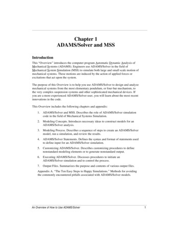
Chapter 1. ADAMS/Solver and MSSFigures 2 and 3 are typical of specific applications for the ADAMS/Solver simulationcode. Figure 2 illustrates a backhoe, while Figure 3 illustrates a satellite with solarpanels.Backhoe Work CycleFigure 2. Backhoe Work CycleFigure 3. Satellite in Orbit About the EarthAn Overview of How to Use ADAMS/Solver5
Chapter 1. ADAMS/Solver and MSSIn Figure 2, ADAMS/Solver simulates part of the work cycle of a backhoe as it digsinto the ground with the bucket, scoops up the dirt, and lifts the dirt. In response toarticulation instructions from the hydraulic systems, ADAMS/Solver computes all ofthe reaction forces on the components of the equipment.The scale for the motion of the backhoe is comparable to its overall dimensions. Theexcitations (movement of the hydraulic cylinders) and applied forces (interactionbetween the bucket and the ground) for the backhoe are highly nonlinear anddependent on the instantaneous state of the mechanical system. These are all typicalcharacteristics of problems for mechanical system simulation.In Figure 3, the gravitational magnetodynamic and aerodynamic forces and momentsaffect the satellite in orbit about the earth. Because of weight restrictions on a satellite,the solar panels are extremely flexible. ADAMS/Solver computes the effects of thepanel flexibility and deformation on the satellite’s overall motion. This information isnecessary to design and verify a control system to maintain the attitude of the principalaxes of the spacecraft as it moves about the earth.1.3.1 Input Specifications for the ADAMS/Solver CodeThe physical laws of mechanical engineering are the basis for the field of MSS. TheMSS simulation tools implement Newton’s laws of motion, or an equivalentformulation of the physical principles. ADAMS/Solver uses the system of EulerLagrange equations of motion. This system, composed of algebraic and second orderdifferential equations, requires sophisticated numerical methods for their solution.ADAMS/Solver defines the following to specify the mechanical model for a simulation: The inertial characteristics of the parts The relationships between parts The driving motions and forces for the systemThe model can also include additional differential (first order) and algebraic equationscoupled to, or independent of, the mechanical system.6An Overview of How to Use ADAMS/Solver
Chapter 1. ADAMS/Solver and MSSThe input data for an ADAMS/Solver simulation includes the following entities: The mass and inertia of the rigid bodies or parts The definition of the geometric aspects of the system including the centers ofmass for the parts, the locations on the parts for the joints that hold the systemtogether, and the points at which the specified motion functions and forcesapply The connectivity for the system (the mechanisms for connecting the parts)defined in terms of mechanical joints, higher-pair contacts, other constraintsand elastic elements A description of the external forces and excitations acting on the system The graphical attributes that enable animation and visualization of the systembehaviorA library of standard joints and higher-pair contacts simplifies the task of defining theconnections between parts of the system.Each ADAMS/Solver simulation begins with an analysis of the input data verifying thatthe description of the mechanical system is Complete Correct ConsistentThe verification process is thorough. A comprehensive set of messages will identifyany errors that can occur in the input data. ADAMS/Solver assembles the differentialand algebraic equations (DAEs) for the actual simulation of the problem only after theinput data passes the above listed standards.An Overview of How to Use ADAMS/Solver7
Chapter 1. ADAMS/Solver and MSS1.3.2 The Analysis ModesADAMS/Solver can perform six different types of analyses depending on thecharacteristics of the problem and the interests that you have. Each of these analysismodes is useful in the appropriate context. As described in the following paragraphs, thevarious analyses provide different information about the system.1.ADAMS/Solver performs an initial conditions analysis (the assembly process)prior to the static, quasi-static, and dynamic analyses. After processing theinput data and before a simulation begins, ADAMS/Solver requires aconsistent set of values for the state of the system. That is, the displacementsand velocities have to satisfy the constraint equations that define the system.Mechanical models frequently involve closed-loop systems that are difficult todefine as illustrated in Figure 4.Slot (Curve)Pin (Point)MFigure 4. Four Bar MechanismIn systems such as this, where M represents applied motion, the state variablesare not all independent. The constraint equations that define the geometricconfiguration of the system also define dependencies between the statevariables. If the displacement and velocity input values are not sufficientlyaccurate, they may not satisfy the constraints in the closed-loop. Therefore,ADAMS/Solver may not recognize some of the system velocities and forces.In complex systems, the initial values that you specify for displacements andvelocities often violate the constraint equations. The initial conditions analysismodifies the input data for the displacements and velocities as needed tosatisfy the system constraints while minimizing the change in the data. Often,it is convenient to specify only a few initial displacements and velocitiesexactly, and allow the initial conditions analysis to assemble the rest of thesystem properly.8An Overview of How to Use ADAMS/Solver
Chapter 1. ADAMS/Solver and MSS2.A kinematic analysis simulates the motion of the system. It allows theengineer to determine the range of possible values for the displacement,velocity, and acceleration of any point of interest on a mechanical device. Ifyou specify the mass and inertial properties of a part, ADAMS/Solver alsocalculates the corresponding applied and reaction forces required to generatethe prescribed motions.The kinematic analysis is algebraic in nature. The implementation inADAMS/Solver is very fast and accurate. Typical applications includedesigning a mechanism for the transfer of motion through a linkage betweenparts and the preliminary examination of a complicated model intended forsubsequent dynamic analyses.3.The static equilibrium analysis determines a state for the system to balance allinternal and external forces in the absence of any system motions or inertialforces. All system velocities and accelerations are set to zero.The analysis for static equilibrium is also algebraic. You often find a startingpoint for a dynamic analysis by using a static analysis to remove unwantedsystem transients at the start of the simulation. Unbalanced forces in the initialconfiguration can generate undesirable effects in the dynamic analysis.4.A quasi-static analysis is a sequence of static analyses performed for differentconfigurations of the system, typically, at fixed time intervals throughout aprescribed motion for the system.5.The most complex and computational demanding mode in ADAMS/Solver isthe dynamic analysis. Several different integrators are available for finding thesolution to the full system of differential and algebraic equations (DAE’s).The dynamic analysis provides the time-history solution for all of thedisplacements, velocities, accelerations, and internal reaction forces in amechanical system driven by a set of external forces and excitations.6.In the linear analysis mode, ADAMS/Solver linearizes the system of nonlinearequations for the model about an operating point. This results in a set of lineartime-invariant (LTI) equations in the formMx·· Cx· Kx Fwhere x represents a perturbation of the state from its operating point; M, C,and K are the equivalent mass, damping, and stiffness matrices, respectively;and F is the column matrix of forcing terms.After ADAMS/Solver computes the various matrices, it performs twodifferent types of linear analyses: eigenanalysis and the generation of statematrices. The eigenanalysis includes the evaluation of both eigenvalues andeigenvectors for the linearized system.An Overview of How to Use ADAMS/Solver9
Chapter 1. ADAMS/Solver and MSSThe eigenvalues are the natural frequencies of the system while theeigenvectors represent the modes of the motion associated with eachfrequency. Generally, both the eigenvalues and the eigenvectors are complexvalued.The state matrices that ADAMS/Solver generates from the linearized systemare the coefficients for a representation of the mechanical system as amultiple-input, multiple-output transfer function in the form·x Ax Buy Cx Duwhere u is the set of inputs and y is the set of outputs. The coefficients A, B,C, and D are the state matrices for the mechanical system.1.3.3 The Output from ADAMS/SolverAt each output time, ADAMS/Solver writes a comprehensive description of the state ofthe system. Thus, a time history can be recorded in the output files. The output includesany combination of the following items if you specify it before running the simulation: Displacements Velocities Accelerations Reaction forces Applied forces User-defined variables User-defined derived results States for system modeling elements Outputs from system modeling elements (such as linear transfer functions) Plant inputs and outputs for the state matrices for a linearized ADAMS/Solvermodel State matrices corresponding to a set of plant inputs and outputs for alinearized ADAMS/Solver model Eigenvalues and eigenvectors at specified operating pointsADAMS/Solver writes the information into a number of output files as described inmore detail in Chapter 7, “Output Files.”10An Overview of How to Use ADAMS/Solver
Chapter 2Modeling ConceptsIntroductionThis chapter is devoted to presenting conceptual material that is unique to MSS andrigid body dynamics. The concepts in this chapter1.Reference Frames. Introduces reference frames and the frames available inADAMS/Solver.2.Coordinate Systems. Defines the difference between coordinate systems andreference frames, and presents the different types of coordinate systemsavailable in ADAMS/Solver.3.Rotation Sequences. Explains why finite rotation sequences are not vectorquantities, why infinitesimal rotation sequences can be represented as vectorquantities, and representation of orientations, in general.4.Location and Orientation Methods. Describes two methods available inADAMS/Solver for locating and orienting coordinate systems.5.Global versus Local Geometric Data. Highlights the differences betweeninputting data relative to the global coordinate system and inputting datarelative to LPRFs.6.Degrees of Freedom. Introduces the concept of degrees of freedom in amechanical system, the redundant constraint handling and overconstraintchecking in ADAMS/Solver, the concept of loops in a mechanical system, theGruebler equation for calculating the degrees of freedom, and the topologicaldata ADAMS/Solver can generate.7.Force Direction and Application. Discusses how ADAMS/Solver directs andapplies forces.An Overview of How to Use ADAMS/Solver11
Chapter 2. Modeling Concepts2.1 Reference FrameA reference frame specifies a reference for the calculation of velocities andaccelerations of a system.2.1.1 Ground Reference FrameThe ground reference frame by definition is the single Newtonian inertial referencethat establishes “absolute rest.” By definition, any point belonging to the groundreference frame has zero velocity and acceleration. It is fixed in “absolute space.”ADAMS/Solver expresses Newton’s Laws in the ground reference frame. For manyapplications, you can consider the Earth as a Newtonian reference frame, even thoughit travels in an elliptical path about the sun (and is therefore accelerating), and rotateson its own axis.2.1.2 Part Reference FramesEvery rigid body has one reference frame called the part reference frame. You can usethe terms “rigid body” and “part reference frames” synonymously.12An Overview of How to Use ADAMS/Solver
Chapter 2. Modeling Concepts2.2 Coordinate SystemsA coordinate system is essentially a measuring stick used to define kinematic anddynamic quantities. Coordinate systems usually consist of an origin and a set of threemutually orthogonal unit vectors that specify three directions. Associated with each ofthese directions is a “scale” that permits measurement of quantities in the coordinatesystem. You can specify all kinematic and kinetic vector quantities as projections ofthe vector along the three unit vectors î, ĵ, and k̂ , as shown in Figure 5.POy R R x i R y j Rz k j iOx kzFigure 5. A Coordinate SystemFigure 5 illustrates a vector R that is defined as the displacement of point P in thecoordinate system OXYZ. Rx, Ry, and Rz are the measure numbers of R along the x, y,and z axes of the coordinate system.Coordinate systems are useful for specifying a model configuration or its velocitiesand accelerations. You can fix coordinate systems to a reference frame or move themwith respect to a reference frame.ADAMS/Solver uses three types of coordinate systems. They are GroundAn Overview of How to Use ADAMS/Solver13
Chapter 2. Modeling Concepts14 Local part reference frame MarkerAn Overview of How to Use ADAMS/Solver
Chapter 2. Modeling Concepts2.2.1 Ground Coordinate SystemThe ground coordinate system rigidly attaches to the ground reference frame or theground part. In ADAMS/Solver, you specify the locations, orientations, and velocitiesof all other rigid bodies or “parts” in the ground coordinate system.2.2.2 Local Part Reference FrameThe Local Part Reference Frame (LPRF) is actually a coordinate system. Every part inADAMS/Solver has a single LPRF. You can specify the initial location and orientationof a part in ADAMS/Solver by specifying the location and orientation of the LPRFwith respect to the ground coordinate system. The LPRF moves with its part. A part'sLPRF defaults to the ground coordinate system whenever you do not specify a LPRF.2.2.3 MarkersA marker is a coordinate system owned by a part. There are two types of markers inADAMS/Solver: fixed and floating.2.2.3.1 Fixed MarkerA fixed marker attaches to a part and moves with that part. To place a marker on a part,you must specify its location and orientation with respect to the LPRF of the part.Markers have many different functions in ADAMS/Solver. They can define thegraphical periphery of a part, locate the part center of mass, provide sites for reactionforce application and joint attachments, or perform other location and orientationfunctions. Certain joints, such as ball-and-socket joints, use the origin of a marker tolocate their centers of action on the parts. Other joints, such as cylindrical joints, usethe z-axes of markers for orienting the translational and/or rotational freedom ofmotion for the parts.2.2.3.2 Floating MarkerSome forces and constraints in ADAMS/Solver use floating markers to specify sitesfor applying forces on parts. You do not specify a fixed position for a floating marker.The force or constraint dictates the position and orientation of the floating marker. Thisposition and orientation can change during the simulation.An Overview of How to Use ADAMS/Solver15
Chapter 2. Modeling Concepts2.3 Rotation SequencesBody-fixed 3-1-3 (Euler angles or z-x-z) rotation sequences are one wayADAMS/Solver allows you to specify part and marker orientations. By default,ADAMS/Solver reports orientations using body-fixed 3-1-3 rotation sequences.Consequently, this section discusses some of the general characteristics of bothrotation sequences and orientation methods.2.3.1 Finite Rotation Sequences are Not Vector QuantitiesKinematics is the study of motions in a system. The displacements, velocities, andaccelerations are the variables of interest. Most of these variables are vector quantities.Thus, it is tempting to try to represent rotation sequences with vectors. Certainly, youcan assign a direction (the axis of rotation) and a magnitude (the angle of rotation). Asthe following analysis shows, however, a finite rotation sequence is not a vector.Suppose α and β are two “rotational vectors” associated with two different axes ofrotation and with transformation matrices A and B. To qualify as elements of a vectorspace, the rotations α and β would have to be commutative. The addition of twoconsecutive rotations corresponds to the product of the two transformation matrices.A B B A, and hence α and β are not commutative in addition, and therefore are notvectors.2.3.2 Infinitesimal Rotation Sequences Can Be Represented asVector QuantitiesLet A and B be two transformation matrices corresponding to a sequence of twoinfinitesimal rotations, that isA I e1where e1 is the change in the transformation matrix due to the first infinitesimal rotation.B I e2where e2 is the change in the transformation matrix due to the second infinitesimalrotation.The addition of two rotations corresponds to the multiplication of the correspondingtransformation matrices, that isA B I e1 e2 e1 e2.Ignoring higher order infinitesimals, one gets:A B I e1 e2 I e2 e1 B A.Infinitesimal rotations are therefore commutative in addition and can be represented asvectors.16An Overview of How to Use ADAMS/Solver
Chapter 2. Modeling ConceptsADAMS/Solver sometimes assumes infinitesimal rotations. For more information,see the discussions of angles under the BEAM, BUSHING, and FIELD statements(Sections 2.5.2, 2.5.3, and 2.5.4, respectively) in the ADAMS/Solver ReferenceManual.2.3.3 Representation of OrientationsA body-fixed 3-1-3 (Euler angle or z-x-z) rotation sequence is one of many ways forrepresenting orientations. In general, the complete representation of an orientationincludes the following: The axis about which each rotation takes place The angle of rotation about each axis The sequence of rotationsA body-fixed 3-1-3 rotation sequence defines each of these. Following is a list of othermethods you can use to represent three-dimensional rotations and the number of valueseach requires. Direction cosines matrix or transformation matrix (9 values) Euler Parameters (4 values) Rodrigues Parameters (3 values)For inputting orientations, ADAMS/Solver permits the use of direction cosines (thex-point and z-point method) and body-fixed 3-1-3 rotation sequences (the Euler anglesmethod). ADAMS/Solver permits numerous methods for outputting orientations. Formore information on the numerous methods available for outputting orientationinformation, see Section 3.4.9, “RCNVRT” in the ADAMS/Solver SubroutinesReference Manual.An Overview of How to Use ADAMS/Solver17
Chapter 2. Modeling Concepts2.4 Location and Orientation MethodsFor locating and orienting any part with respect to the ground coordinate system or anymarker with respect to its LPRF, you can use one of three methods: Euler angles method X-point-z-point method (also known as the direction cosines method)Since you use these methods to locate and orient both LPRFs and markers, we refer tothe coordinate systems that you locate and orient as “positioned frames” and to thecoordinate systems with respect to which you locate and orient them as “base frames.”For example, if you orient a part with respect to the ground coordinate system, the partis the positioned frame and the ground coordinate system is the base frame. Similarly,if you orient a marker with respect to a LPRF, the marker is the positioned frame, andthe LPRF is the base frame.2.4.1 Euler Angles MethodWhen you use the Euler angles method to locate and orient a positioned frame withrespect to a base frame, specify the following geometric data: Cartesian coordinates to define the origin of the positioned frame with respectto the base frame Body-fixed 3-1-3 Euler angles to define the orientation of the positionedframe with respect to the base frame.Since Euler angle rotations cumulatively define the orientation of the positioned frame,you may find it difficult to envision orientations that involve rotations of other than0-, 45-, or 90- degree increments. When orienting a reference frame that requires acomplex combination of rotations, you may find it more convenient to use thex-point-z-point orientation method (see Section 2.4.2, “X-Point-Z-Point Method”).18An Overview of How to Use ADAMS/Solver
Chapter 2. Modeling Concepts2.4.2 X-Point-Z-Point MethodYou can use the x-point-z-point method to specify the location of the positioned framerelative to the base frame and the orientation (in direction cosines) of the positionedframe relative to the base frame. The x point defines the x-axis or the first column ofthe direction cosines matrix, and the z point defines the z-axis or the third column ofthe direction cosines matrix. ADAMS/Solver calculates the y-axis or the secondcolumn using the orthogonal properties of transformation matrices.When you use the x-point-z-point method to locate and orient a positioned frame,provide the following geometric data with respect to the base frame: Cartesian coordinates of the positioned frame origin (point Q) Cartesian coordinates of a point on the z-axis of the positioned frame(point Z) or of a point on the x-axis of the positioned frame (point X). Providea point on the z-axis when it is important to exactly specify the z-axis of thepositioned frame. Provide the Cartesian coordinates of a point on the x-axiswhen it is important to exactly specify the x-axis of the positioned frame. Cartesian coordinates of a point that is in the x-z plane of the positionedframe. If you provided a point on the z-axis of the positioned frame (point Z),the point in the x-z plane should be noncollinear with points Q and Z (that is,provide point X). If you provided a point on the x-axis of the positioned frame(point X), the point in the x-z plane should be noncollinear with points Q andX (that is, provide point Z).For orienting a marker with respect to a LPRF, ADAMS/Solver refers to the threepoints as QP, ZP, and XP, respectively. For orienting a LPRF with respect to theground reference frame, ADAMS/Solver refers to the three points as QG, ZG, and XG,respectively. Figure 6 shows the Q, Z, and X points and their coordinates with respectto the base frame. If vectors QZ and QX are not orthogonal, ADAMS/Solver redirectseither QX or QZ so that they are orthogonal. Note that in Figure 6, a point on the z-axisof the positioned frame specifies exactly the z-axis of the frame.An Overview of How to Use ADAMS/Solver19
Chapter 2. Modeling qx,qy,qz)yBaseFramezxFigure 6. X-Point-Z-Point MethodBy default, ADAMS/Solver assumes that Q defines the exact location of the frameorigin and that Z defines an exact axis orientation. Because the third point (X bydefault) does not necessarily lie on an axis, ADAMS/Solver determines the vectorcross product of vectors QZ and QX to form an orthogonal y-axis. Then,ADAMS/Solver determines the vector cross product of the new y-axis and the exactaxis (the z-axis by default) to produce the orientation of the remaining axis.20An Overview of How to Use ADAMS/Solver
Chapter 2. Modeling Concepts2.5 Global Versus Local Geometric DataRegardless of the comb
MSS can incorporate data from other software products into a complete simulation of system behavior. MSS also produces output that assists in further analysis with other computational tools. As Figure 1 illustrates, MSS software exchanges data with other applications. A discussion of these applications follows Figure 1.