Transcription
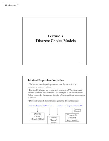
RS – Lecture 17Lecture 3Discrete Choice Models1Limited Dependent Variables To date we have implicitly assumed that the variable yi is acontinuous random variable. But, the CLM does not require this assumption! The dependentvariable can have discontinuities. For example, it can be discrete orfollow counts. In these cases, linearity of the conditional expectationsis unusual. Different types of discontinuities generate different models:Discrete Dependent VariableContinuous dependent variableTruncated,CensoredDiscreteChoiceModels (DCM)Duration(Hazard)ModelsTruncated/CensoredRegr. Models
RS – Lecture 17Limited Dependent VariablesWith limited dependent variables, the conditional mean is rarelylinear. We need to use adjusted models.From Frances and Paap (2001)Limdep: Discrete Choice Models (DCM) We usually study discrete data that represent a decision, a choice. Sometimes, there is a single choice. Then, the data come in binaryform with a ”1” representing a decision to do something and a ”0”being a decision not to do something. Single Choice (binary choice models): Binary DataData:yi 1 (yes/accept) or 0 (no/reject)- Examples: Trade a stock or not, do an MBA or not, etc. Or we can have several choices. Then, the data may come as 1, 2,., J, where J represents the number of choices. Multiple Choice (multinomial choice models)Data:yi 1(opt. 1), 2 (opt. 2), ., J (opt. J)- Examples: CEO candidates, transportation modes, etc.
RS – Lecture 17Limdep: DCM – Binary Choice - ExampleLimdep: DCM – Mulinomial Choice - ExampleFlyGround
RS – Lecture 17Limdep: Truncated/Censored Models Truncated variables:We only sample from (observe/use) a subset of the population.The variable is observed only beyond a certain threshold level(‘truncation point’)- store expenditures, labor force participation, income belowpoverty line. Censored variables:Values in a certain range are all transformed to/grouped into (orreported as) a single value.- hours worked, exchange rates under Central Bank intervention.Note: Censoring is essentially a defect in the sample data. Presumably,if they were not censored, the data would be a representativesample from the population of interest.Limdep: Censored Health Satisfaction Data0 Not Healthy1 Healthy
RS – Lecture 17Limdep: Duration/Hazard Models We model the time between two events.Examples:– Time between two trades– Time between cash flows withdrawals from a fund– Time until a consumer becomes inactive/cancels a subscription– Time until a consumer responds to direct mail/ a questionnaireMicroeconomics behind Discrete Choice Consumers Maximize Utility. Fundamental Choice Problem:Max U(x1,x2, ) subject to prices and budget constraints A Crucial Result for the Classical Problem:– Indirect Utility Function: V V(p,I)– Demand System of Continuous Choicesx*j V (p, I) / p j V (p, I) / I The Integrability Problem: Utility is not revealed by demands
RS – Lecture 17Theory for Discrete Choice Theory is silent about discrete choices Translation to discrete choice- Existence of well defined utility indexes: Completeness of rankings- Rationality: Utility maximization- Axioms of revealed preferences Choice and consideration sets: Consumers simplify choice situations Implication for choice among a set of discrete alternatives Commonalities and uniqueness– Does this allow us to build “models?”– What common elements can be assumed?– How can we account for heterogeneity? Revealed choices do not reveal utility, only rankings which are scaleinvariant.Discrete Choice Models (DCM) We will model discrete choice. We observe a discrete variable yiand a set of variables connected with the decision xi, usually calledcovariates. We want to model the relation between yi and xi. It is common to distinguish between covariates zi that vary byunits (individuals or firms), and covariates that vary by choice (andpossibly by individual), wij. Example of zi‘s: individual characteristics, such as age or education. Example of wij: the cost associated with the choice, for example thecost of investing in bonds/stocks/cash, or the price of a product. This distinction is important for the interpretation of these modelsusing utility maximizing choice behavior. We may put restrictionson the way covariates affect utilities: the characteristics of choice ishould affect the utility of choice i, but not the utility of choice j.
RS – Lecture 17Discrete Choice Models (DCM) The modern literature goes back to the work by Daniel McFaddenin the seventies and eighties (McFadden 1973, 1981, 1982, 1984). Usual Notation:n decision makeri,j choice optionsy decision outcomex explanatory variables/covariatesβ parametersε error termI[.] indicator function: equal to 1 if expression within brackets istrue, 0 otherwise. Example: I[y j x] 1 if j was selected (given x) 0 otherwiseDCM – What Can we Learn from the Data? Q: Are the characteristics of the consumers relevant? Predicting behavior- Individual – for example, will a person buy the add-on insurance?- Aggregate – for example, what proportion of the population willbuy the add-on insurance? Analyze changes in behavior when attributes change. For example,how will changes in education change the proportion of who buy theinsurance?
RS – Lecture 17Application: Health Care Usage (Greene)German Health Care Usage Data, N 7,293, Varying Numbers of PeriodsData downloaded from Journal of Applied Econometrics Archive. This is anunbalanced panel with 7,293 individuals. This is a large data set. There are altogether27,326 observations. The number of observations ranges from 1 to 7. (Frequenciesare: 1 1525, 2 2158, 3 825, 4 926, 5 1051, 6 1000, 7 987). (Downloaded fromthe JAE Archive)Variables in the file C HHKIDSEDUCAGEFEMALEEDUC 1(Number of doctor visits 0)1(Number of hospital visits 0)health satisfaction, coded 0 (low) - 10 (high)number of doctor visits in last three monthsnumber of hospital visits in last calendar yearinsured in public health insurance 1; otherwise 0insured by add-on insurance 1; otherswise 0household nominal monthly net income in German marks / 10000.(4 observations with income 0 were dropped)children under age 16 in the household 1; otherwise 0years of schoolingage in years1 for female headed household, 0 for maleyears of educationApplication: Binary Choice Data (Greene)
RS – Lecture 17Application: Health Care Usage (Greene)Q: Does income affect doctor’s visits? What is the effect of age ondoctor’s visits? Is gender relevant?27,326 Observations –– 1 to 7 years, panel– 7,293 households observed– We use the 1994 year 3,337 household observationsDescriptive Statistics VariableMeanStd.Dev.MinimumMaximum-------- TOR .657980.474456.0000001.00000AGE 42.626611.586025.000064.0000HHNINC .444764.216586.340000E-01 3.00000FEMALE .463429.498735.0000001.00000DCM: Setup – Choice Set1. Characteristics of the choice set- Alternatives must be mutually exclusive: No combination ofchoice alternatives. For example, no combination of differentinvestments types (bonds, stocks, real estate, etc.).- Choice set must be exhaustive: all relevant alternatives included.If we are considering types of investments, we should include all:bonds; stocks; real estate; hedge funds; exchange rates;commodities, etc. If relevant, we should include international anddomestic financial markets.- Finite (countable) number of alternatives.
RS – Lecture 17DCM: Setup – RUM2. Random utility maximization (RUM)Assumption: Revealed preference. The decision maker selects thealternative that provides the highest utility. That is,Decision maker n selects choice i if Uni Unj j iDecomposition of utility: A deterministic (observed), Vnj, and random(unobserved) part, εnj:Unj Vnj εnj- The deterministic part, Vnj, is a function of some observed variables,xnj (age, income, sex, price, etc.):Vnj α β1 Agen β2 Incomenj β3 Sexn β4 Pricenj- The random part, εnj, follows a distribution. For example, a normal.DCM: Setup – RUM2. Random utility maximization (RUM) We think of an individual’s utility as an unobservable variable, withan observable component, V, and an unobservable (tastes?) randomcomponent, ε. The deterministic part is usually intrinsic linear in the parameters.Vnj α β1 Agen β2 Incomenj β3 Sexn β4 Pricenj- In this formulation, the parameters, β, are the same for allindividuals. There is no heterogeneity. This is a useful assumption forestimation. It can be relaxed.
RS – Lecture 17DCM: Setup - RUM2. Random utility maximization (continuation)Probability Model: Since both U’s are random, the choice is random.Then, n selects i over j if:P ni Prob(U Prob(Vni εni Vnj εnj j i) Prob(εnj εni Vni Vnj j i) njP ni I (ε Uni εninj j i) V ni V nj j i ) f ( ε n ) d εn Pnj F(X,β) is a CDF. Vnj - Vnj h(X, β). h(.) is usually referred as the index function. To evaluate the CDF, F(X,β), f(εn) needs to be specified.DCM: Setup - RUM1F h ( xi , β ) Pr [ yi 1]0h(X, β).
RS – Lecture 17DCM: Setup - RUM To evaluate the integral, f(εn) needs to be specified. Manypossibilities:– Normal:Probit Model, natural for behavior.– Logistic: Logit Model, allows “thicker tails.”– Gompertz: Extreme Value Model, asymmetric distribution. We can use non-parametric or semiparametric methods to estimatethe CDF F(X,β). These methods impose weaker assumptions thanthe fully parametric model described above. In general, there is a trade-off: Less assumptions, weakerconclusions, but likely more robust results.DCM: Setup – RUM – Different f(εn)
RS – Lecture 17DCM: Setup - RUM Note: Probit? Logit?A one standard deviation change in the argument of a standardNormal distribution function is usually called a “Probability Unit” orProbit for short. “Probit” graph papers have a normal probabilityscales on one axis. The Normal qualitative choice model becameknown as the Probit model. The “it” was transmitted to the LogisticModel (Logit) and the Gompertz Model (Gompit).DCM: Setup - Distributions Many candidates for CDF –i.e., Pn(x’nβ) F(Zn),:– Normal (Probit Model) Φ(Zn)– Logistic (Logit Model) 1/[1 exp(-Zn)]– Gompertz (Gompit Model) 1 – exp[-exp(Zn)] Suppose we have binary (0,1) data. Assume β 0.- Probit Model: Prob(yn 1) approaches 1 very rapidly as X andtherefore Z increase. It approaches 0 very rapidly as X and Z decrease- Logit Model: It approaches the limits 0 and 1 more slowly thandoes the Probit.- Gompit Model: Its distribution is strongly negatively skewed,approaching 0 very slowly for small values of Z, and 1 even morerapidly than the Probit for large values of Z.
RS – Lecture 17DCM: Setup - Distributions Comparisons: Probit vs LogitDCM: Setup - NormalizationNote: Not all the parameters may be identified. Suppose we are interested in whether an agent chooses to visit adoctor or not –i.e., (0,1) data. If Uvisit 0, an agent visits a doctor.Uvisit 0 α β1 Age β2 Income β3 Sex ε 0 ε -(α β1 Age β2 Income β3 Sex)Let Y 1 if Uvisit 0Var[ε] σ2 Now, divide everything by σ.Uvisit 0 ε/σ -[α/σ (β1/σ) Age (β2/σ)Income (β3/σ) Sex] 0orw -[α’ β1’Age β’Income β’Sex] 0
RS – Lecture 17DCM: Setup - Normalization Dividing everything by σ.Uvisit 0 ε/σ -[α/σ (β1/σ) Age (β2/σ)Income (β3/σ) Sex] 0orw -[α’ β1’Age β’Income β’Sex] 0Y 1 if Uvisit 0Var[w] 1Same data. The data contain no information about the variance. Wecould have assigned the values (1,2) instead of (0,1) to yn. It ispossible to produce any range of values in yn. Normalization: Assume Var[ε] 1.DCM: Setup - AggregationNote: Aggregation can be problematic- Biased estimates when aggregate values of the explanatory variablesare used as inputs:E P1 ( x ) P1 E ( x ) - But, when the sample is exogenously determined, consistentestimates can be obtained by sample enumeration:- Compute probabilities/elasticities for each decision maker- Compute (weighted) average of these values.1P1 P1 ( xi )N i More on this later.
RS – Lecture 17DCM: Setup – AggregationExample (from Train (2002)): Suppose there are two types ofindividuals, a and b, equally represented in the population, withVa β ′xaVb β ′xbthenPb Pr yi 1 xb Pa Pr yi 1 xa F [ β ′xb ] F [ β ′xa ]butP 12( Pa Pb ) P ( x ) F [ β ′x ]DCM: Setup – AggregationIn general, P (V ) will tend to (underestimate) overestimate Pwhen probabilities are (high) lowF ( )PbPP (V )PaVaVVbV
RS – Lecture 17DCM: Setup - AggregationGraph: Average probability (2.1) vs. Probability of the average (2.2)DCM: Setup - Identification3. Identification problemsa. Only differences in utility matterChoice probabilities do not change when a constant is added to eachalternative’s utilityImplication: Some parameters cannot be identified/estimated.Alternative-specific constants; coefficients of variables thatchange over decision makers but not over alternatives.b. Overall scale of utility is irrelevantChoice probabilities do not change when the utility of all alternativesare multiplied by the same factorImplication: Coefficients of different models (data sets) are notdirectly comparable.Normalization of parameters or variance of error terms is used todeal with identification issues.
RS – Lecture 17DCM: Estimation Since we specify a pdf, ML estimation seems natural to do. But, ingeneral, it can get complicated. In general, we assume the following distributions:– Normal:Probit Model Φ(x’nβ)– Logistic:Logit Model exp(x’nβ)/[1 exp(x’nβ)]– Gompertz: Extreme Value Model 1 – exp[-exp(x’nβ)] Methods- ML estimation (Numerical optimization)- Bayesian estimation (MCMC methods)- Simulation-assisted estimationDCM: ML Estimation Example: Logit ModelSuppose we have binary (0,1) data. The logit model follows from:Pn[yn 1 x] exp(x’nβ)/[1 exp(x’nβ) F(x’nβ)Pn[yn 0 x] 1/[1 exp(x’nβ)] 1 - F(x’nβ)- Likelihood functionL(β) Πn (1- P [yn 1 x,β]) P[yn 1 x,β]- Log likelihoodLog L(β) Σy 0 log[1- F(x’nβ)] Σy 1 log[F(x’nβ)]- Numerical optimization to get β. The usual problems with numerical optimization apply. Thecomputation of the Hessian, H, may cause problems. ML estimators are consistency, asymptotic normal and efficient.
RS – Lecture 17DCM: ML Estimation Example: Logit ModelSuppose we have binary (0,1) data. The logit model follows from:Pn[yn 1 x] exp(x’nβ)/[1 exp(x’nβ) F(x’nβ)Pn[yn 0 x] 1/[1 exp(x’nβ)] 1 - F(x’nβ)- Likelihood functionL(β) Πn (1- P [yn 1 x,β]) P[yn 1 x,β]- Log likelihoodLog L(β) Σy 0 log[1- F(x’nβ)] Σy 1 log[F(x’nβ)]- Numerical optimization to get β. The usual problems with numerical optimization apply. Thecomputation of the Hessian, H, may cause problems. ML estimators are consistency, asymptotic normal and efficient.DCM: ML Estimation – Covariance Matrix How can we estimate the covariance matrix, Σβl?Using the usual conditions, we can use the information matrix: 2L I n g e n e r a l: Σ β l E β β′ 1 I (β ) 1 1N e w to n -R a p h s o n : Σ β l 2L β β′ β βl 1 T L i L i B H H H : Σ βl i 1 β β ′ β β l The NR and BHHH are asymptotically equivalent but in smallsamples they often provide different covariance estimates for thesame model38
RS – Lecture 17DCM: ML Estimation Numerical optimization - Steps:(1) Start by specifying the likelihood for one observation: Fn(X,β)(2) Get the joint likelihood function: L(β) Πn Fn(X,β)(3) It is easier to work with the log likelihood function:Log L(β) Σ n ln(Fn(X,β))(4) Maximize Log L(β) with respect to β- Set the score equal to 0 no closed-form solution- Numerical optimization, as usual:(i) Starting values β0(ii) Determine new value βt 1 βt update, such that LogL(βt 1) Log L(βt).Say, N-R’s updating step:βt 1 βt - λt H-1 f (βt)(iii) Repeat step (ii) until convergence.DCM: Bayesian Estimation The Bayesian estimator will be the mean of the posterior density:f (β , γ y , X ) f ( y X, β, γ ) f (β, γ ) f ( y X, β, γ )f ( y X, β, γ ) f (β, γ ) f (y X, β, γ) f (β, γ )dβdγ- f(β,γ) is the prior density for the model parameters- f( y X,β,γ) is the likelihood. As usual we need to specify the prior and the likelihood:- The priors are usually non-informative (flat), say f(β,γ) α 1.- The likelihood depends on the model in mind. For a Probit Model,we will use a normal distribution. If we have binary data, then,f( y X,β,γ) Πn (1-Φ[yn x,β,γ]) Φ[yn x,β,γ]
RS – Lecture 17DCM: Bayesian Estimation Let θ (β,γ). Suppose we have binary data with Pn[yn 1 x, θ] F(x’n,,θ). The estimator of θ is the mean of the posterior density.Under a flat prior assumption:N f (y X, θ) f (θ) dθ (1 F ( X, θ))θθ f ( y X, θ ) f ( θ ) d θE [θ y , X ] yn( F ( X, θ )) y n d θn 1N (1 F ( X, θ))yn( F ( X, θ )) y n d θn 1 Evaluation of the integrals is complicated. We will evaluate themusing MCMC methods. Much simpler.MP Model – Simulation-based Estimation ML Estimation is likely complicated due to the multidimensionalintegration problem. Simulation-based methods approximate theintegral. Relatively easy to apply. Simulation provides a solution for dealing with problems involvingan integral. For example:E[h(U)] h(u) f(u) du All GMM and many ML problems require the evaluation of anexpectation. In many cases, an analytic solution or a precise numericalsolution is not possible. But, we can always simulate E[h(u)]:- Steps- Draw R pseudo-RV from f(u): u1, u2, .,uR(R: repetitions)- Compute Ê[h(U)] (1/R) Σn h(un)
RS – Lecture 17MP Model – Simulation-based Estimation We call Ê[h(U)] a simulator. If h(.) is continuous and differentiable, then Ê[h(U)] will becontinuous and differentiable. Under general conditions, Ê[h(U)] provides an unbiased (& most ofthe times consistent) estimator for E[h(U)]. The variance of Ê[h(U)] is equal to Var[h(U)]/R. There are many simulators. But the idea is the same: compute anintegral by drawing pseudo-RVs, never by integration.DCM: Partial Effects In general, the β’s do not have an interesting interpretation. βk doesnot have the usual marginal effect interpretation. To make sense of β’s, we calculate:Partial effect P(α β1Income )/ xk (derivative)Marginal effect E[yn x]/ xkElasticity log P(α β1Income )/ log xk Partial effect x xk/P(α β1Income ) These effects vary with the values of x: larger near the center of thedistribution, smaller in the tail. To calculate standard errors for these effects, we use delta method.
RS – Lecture 17DCM: Partial Effects – Delta Method We know the distribution of bn, with mean θ and variance σ2/n, butwe are interested in the distribution of g(bn), where (g(bn) is acontinuous differentiable function, independent of n.) After some work (“inversion”), we obtain:g(bn) N(g(θ), [g′(θ)]2 σ2/n).aWhen bn is a vector,g(bn)a N(g(θ), [G(θ)]’ Var[bn] [G(θ)]).where [G(θ)] is the Jacobian of g(.). In the DCM case, g(bn) F(x’nβ). Note: A bootstrap can also be used.DCM: Partial Effects – Sample Means or Average The partial and marginal effects will vary with the values of x. It is common to calculate these values at, say, the sample means ofthe x. For example:Estimated Partial effect f (α β1Mean(Income) )-f(.) pdf The marginal effects can also be computed as the average of themarginal effects at every observation. In principle, different models will have different effects. Practical Question: Does it make a difference the P(.) used?
RS – Lecture 17DCM: Goodness of Fit Q: How well does a DCM fit?In the regression framework, we used R2. But, with DCM, there areno residuals or RSS. The model is not computed to optimize thefit of the model: There is no R2. “Fit measures” computed from log L- Let Log L(β0) only with constant term. Then, define Pseudo R²:Pseudo R² 1 – Log L(β)/Log L(β0) (“likelihood ratio index”)(This McFadden’s Pseudo R² . There are many others.)- LR-test : LR -2(Log L(β0) – Log L(β)) χ²(k)- Information Criterion: AIC, BIC sometimes conflicting resultsDCM: Goodness of Fit “Fit measures” computed from accuracy of predictionsDirect assessment of the effectiveness of the model at predicting theoutcome –i.e., a 1 or a 0.- Computation- Use the model to compute predicted probabilities- Use the model and a rule to compute predicted y 0 or 1Rule: Predict y 1 if estimated F is “large”, say 0.5 or greaterMore general, use ŷ 1 if estimated F is greater than P*Example: Cramer Fit measureF̂ Predicted ProbabilityΣ N y Fˆ Σ N (1 yi )Fˆλˆ i 1 i i 1N1N0λˆ M ean Fˆ when y 1-Mean Fˆ when y 0 reward for correct predictions minuspenalty for incorrect predictions
RS – Lecture 17Cross Tabulation of Hits and MissesLet 1yˆ i 0Fˆi 0.5Fˆi 0.5PredictedFˆi 0.5ActualFˆi 0.5yi 1yi 0 The prediction rule is arbitrary.– No weight to the costs of individual errors made. It may be morecostly to make an error to classify a “yes” as a “no” than viceversa.– In this case, some loss functions would be more helpful than others. There is no way to judge departures from a diagonal table.DCM: Model Selection Model selection based on nested models: Use the Likelihood:- LR-testLR -2(Log L(βr) – Log L(βu))r restricted model; u unrestricted (full) modelLR χ²(k) (k difference in # of parameters) Model selection based for non-nested models: AIC, CAIC, BIC lowest value
RS – Lecture 17DCM: Testing Given the ML estimation setup, the trilogy of tests (LR, W, and LM)is used:- LR Test: Based on unrestricted and restricted estimates.- Distance Measures - Wald test: Based on unrestricted estimates.- LM tests: Based on restricted estimates. Chow Tests that check the constancy of parameters can be easilyconstructed.- Fit an unrestricted model, based on model for the differentcategories (say, female and male) or subsamples (regimes), andcompare it to the restricted model (pooled model) LR test.DCM: Testing Issues:- Linear or nonlinear functions of the parameters- Constancy of parameters (Chow Test)- Correct specification of distribution- Heteroscedasticity Remember, there are no residuals. There is no F statistic.
RS – Lecture 17DCM: Heteroscedasticity In the RUM, with binary data agent n selectsyn 1 iffUn β’xn εn 0,where the unobserved εn has E[εn] 0, and Var[εn] 1 Given that the data do not provide information on σ, we assumevariance 1, an identification assumption. But, implicitly we areassuming homoscedasticity across individuals. Q: Is this a good assumption? The RUM framework resembles a regression, where in thepresense of heteroscedasticity, we scale each observation by thesquared root of its variance.DCM: Heteroscedasticity Q: How to accommodate heterogeneity in a DCM?Use different scaling for each individual. We need to know themodel for the variance.– Parameterize: Var[εn] exp(zn γ)– Reformulate probabilitiesBinary Probit or Logit: Pn[yn 1 x] P(xn β/exp(zn γ)) Marginal effects (derivative of E[yn] w.r.t. xn and zn) are now morecomplicated. If xn zn, signs and magnitudes of marginal effectstend to be ambiguous.
RS – Lecture 17DCM: Heteroscedasticity - Testing There is no generic, White-type test for heteroscedasticity. We dothe tests in the context of the maximum likelihood estimation. Likelihood Ratio, Wald and Lagrange Multiplier Tests are allstraightforward All heteroscedasticity tests require a specification of the modelunder H1 (heteroscedasticity), say,H1: Var[εn] exp(zn γ)DCM: Robust Covariance Matrix (Greene) In the context of maximum likelihood estimation, it is common todefine the Var[bM] (1/T) H0-1V0 H0-1 , where if the model iscorrectly specified: -H V. Similarly, for a DCM we can define:"Robust" Covariance Matrix: V A B AA negative inverse of second derivatives matrix 12 2 log L N log Prob i estimated E i 1 βˆ βˆ ′ β β ′ B matrix sum of outer products of first derivatives 1 log L log L estimated E β ′ βFor a logit model, A B log Prob i log Prob i i 1 βˆ βˆ ′ NPˆ (1 Pˆi ) x i x ′i i 1 i N 1 N( yi Pˆi ) 2 x i x ′i i 1 ei2 x i x ′i (Resembles the White estimator in the linear model case.)Ni 1 1
RS – Lecture 17DCM: Robust Covariance Matrix (Greene) Q: Is this matrix robust to what? It is not “robust” to:– Heteroscedasticity– Correlation across observations– Omitted heterogeneity– Omitted variables (even if orthogonal)– Wrong distribution assumed– Wrong functional form for index function In all cases, the estimator is inconsistent so a “robust” covariancematrix is pointless. (In general, it is merely harmless.)DCM: Endogeneity It is possible to have in a DCM endogenous covariates. Forexample, many times we include education as part of an individual’scharacteristics or the income/benefits generated by the choice as partof its characteristics. Now, we divide the covariates in endogenous and exogenous.Suppose agent n selects yn 1 iffUn xn’β hn’θ εn 0,where E[ε h] 0 (h is endogenous) There are two cases:– Case 1: h is continuous (complicated)– Case 2: h is discrete, say, binary. (Easier, a treatment effect)
RS – Lecture 17DCM: Endogeneity Approaches- Maximum Likelihood (parametric approach)- GMM- Various approaches for case 2. Case 2 is the easier case: SE DCM! Concentrate on Case 1 (h is continuous).The usual problems with endogenous variables are made worse innonlinear models. In a DCM is not clear how to use IVs. If moments can be formulated, GMM can be used. For example, ina Probit Model:E[(yn-Φ(xn’β))(xn z)] 0 This moment equation forms the basis of a straightforward twostep GMM estimator. Since we specify Φ(.), it is parametric.DCM: Endogeneity - ML ML estimation requires full specification of the model, including theassumption that underlies the endogeneity of hn. For example:- RUM:Un xn’β hn’θ εn- Revealed preference: yn 1[Un 0]- Endogenous variable: hn zn’α un,withE[ε h] 0 Cov[u,ε] 0 (ρ Corr[u,ε])- Additional Assumptions:1)2) z IV, a valid set of exogenous variables, uncorrelated with (u,ε) ML becomes a simultaneous equations model.
RS – Lecture 17DCM: Endogeneity - ML ML becomes a simultaneous equations model.- Reduced form estimation is possible:- Insert the second equation in the first. If we use a Probit Model,this becomes Prob(yn 1 xn,zn) Φ(xn′β* zn′α*).- FIML is probably simpler:- Write down the joint density:f(yn xn,zn) f(zn).- Assume probability model for f(yn xn,zn), say a Probit Model.- Assume marginal for f(zn), say a normal distribution.- Use the projection: εn un [(ρσ)/σu2] un vn,σv2 (1- ρ2).- Insert projection in P(yn)- Replace un (hn - zn’α) in P(yn).- Maximize Log L(.) w.r.t. (β,α,θ,ρ,σu)DCM: Endogeneity – ML: Probit (Greene)P robit fit of y to x and h w ill not consistently estim ate ( β , θ )because of the correlation betw een h and ε induced by thecorrelation of u and ε . U sing the bivariate norm ality, β ′x θ h ( ρ / σ ) u u P rob ( y 1 x , h ) Φ 2 1 ρInsertu i ( hi - α ′z )/ σ u and include f(h z ) to form logLlogL hi - α ′z i β ′ x i θ hi ρ σu (2 y 1) logΦi 2N 1 ρ i 1 log 1 φ hi - α ′z i σ u σu
RS – Lecture 17DCM: Endogeneity – ML: 2-Step LIML Two step limited information ML (Control Function) is alsopossible:- Use OLS to estimate α,σu- Compute the residual vn.- Plug residuals vn into the assumed model P(yn)- Fit the probability model for P(yn).- Transform the estimated coefficients into the structural ones.- Use delta method to calculate standard errors.
Sometimes, there is a single choice. Then, the data come in binary form with a ”1”representing a decision to do something and a ”0” being a decision not to do something. Single Choice (binary choice models): Binary Data Data: yi 1 (yes/accept) or 0 (no/rejec