WIXLIB

Figure 2. Richard Feynman and other physicists gathered in June 1947 at ShelterIsland, New York, several months before the meeting at the Pocono Manor Inn inwhich Feynman introduced his diagrams. Standing are Willis Lamb (left) and JohnWheeler. Seated, from left to right, are Abraham Pais, Richard Feynman, HermannFeshbach and Julian Schwinger. (Photograph courtesy of the Emilio Segrè VisualArchives, American Institute of Physics.)Figure 3. Electron-electron scattering is described byone of the earliest published Feynman diagrams (featured in “Sightings,” September–October 2003). Oneelectron (solid line at bottom right) shoots out a forcecarrying particle—a virtual photon (wavy line)—whichthen smacks into the second electron (solid line at bottom left). The first electron recoils backward, while thesecond electron gets pushed off its original course. Thediagram thus sketches a quantum-mechanical view ofhow particles with the same charge repel each other. Assuggested by the term “Space-Time Approach” in thetitle of the article that accompanied this diagram, Feynman originally drew diagrams in which the dimensionswere space and time; here the horizontal axis representsspace. Today most physicists draw Feynman diagramsin a more stylized way, highlighting the topology ofpropagation lines and vertices. (This diagram and Figure 4 are reproduced from Feynman 1949a, by permission of the American Physical Society.)158American Scientist, Volume 93interwar architects of QED knew that they couldapproximate this infinitely complicated calculation because the charge of the electron (e) is sosmall: e2 1/137, in appropriate units. The chargeof the electrons governed how strong their interactions would be with the force-carryingphotons: Every time a pair of electrons tradedanother photon back and forth, the equationsdescribing the exchange picked up another factor of this small number, e 2 (see facing page). Soa scenario in which the electrons traded onlyone photon would “weigh in” with the factor e2,whereas electrons trading two photons wouldcarry the much smaller factor e 4. This event, thatis, would make a contribution to the full calculation that was less than one one-hundredth thecontribution of the single-photon exchange. Theterm corresponding to an exchange of three photons (with a factor of e 6) would be ten thousandtimes smaller than the one-photon-exchangeterm, and so on. Although the full calculationsextended in principle to include an infinite number of separate contributions, in practice anygiven calculation could be truncated after onlya few terms. This was known as a perturbativecalculation: Theorists could approximate the fullanswer by keeping only those few terms thatmade the largest contribution, since all of theadditional terms were expected to contributenumerically insignificant corrections.Deceptively simple in the abstract, thisscheme was extraordinarily difficult in practice. One of Heisenberg’s graduate studentshad braved an e4 calculation in the mid1930s—just tracking the first round of correction terms and ignoring all others—and quickly found himself swimming in hundreds ofdistinct terms. Individual contributions to theoverall calculation stretched over four or fivelines of algebra. It was all too easy to conflateor, worse, to omit terms within the algebraicmorass. Divergence difficulties, acute accounting woes—by the start of World War II, QEDseemed an unholy mess, as calculationally intractable as it was conceptually muddled.Feynman’s RemedyIn his Pocono Manor Inn talk, Feynman toldhis fellow theorists that his diagrams offerednew promise for helping them march throughthe thickets of QED calculations. As one of hisfirst examples, he considered the problem ofelectron-electron scattering. He drew a simplediagram on the blackboard, similar to the onelater reproduced in his first article on the newdiagrammatic techniques (see Figure 3). Thediagram represented events in two dimensions: space on the horizontal axis and time onthe vertical axis.The diagram, he explained, provided ashorthand for a uniquely associated mathematical description: An electron had a certainlikelihood of moving as a free particle from the 2005 Sigma Xi, The Scientific Research Society. Reproductionwith permission only. Contact perms@amsci.org.

point x1 to x5. Feynman called this likelihoodK (5,1). The other incoming electron movedfreely—with likelihood K (6,2)—from pointx2 to x6. This second electron could then emita virtual photon at x6, which in turn wouldmove—with likelihood δ (s562)—to x5, wherethe first electron would absorb it. (Here s56represented the distance in space and time thatthe photon traveled.)The likelihood that an electron would emitor absorb a photon was eγµ, where e was theelectron’s charge and γµ a vector of Dirac matrices (arrays of numbers to keep track of theelectron’s spin). Having given up some of itsenergy and momentum, the electron on theright would move from x6 to x4, much the way ahunter recoils after firing a rifle. The electron onthe left, meanwhile, upon absorbing the photon and hence gaining some additional energyand momentum, would scatter from x5 to x3. InFeynman’s hands, then, this diagram stood infor the mathematical expression (itself writtenin terms of the abbreviations K and δ ):e2 d4x5d4x6K (3,5)K (4,6)γµδ (s562)γµK (5,1)K (6,2)In this simplest process, the two electronstraded just one photon between them; thestraight electron lines intersected with the wavyphoton line in two places, called “vertices.”The associated mathematical term thereforeDoing Physics with Feynman DiagramsFeynman diagrams are a powerful tool for making calculations in quantum theory. As in any quantum-mechanicalcalculation, the currency of interest is a complex number, or“amplitude,” whose absolute square yields a probability. Forexample, A(t, x) might represent the amplitude that a particlewill be found at point x at time t; then the probability of finding the particle there at that time will be A(t, x) 2.In QED, the amplitudes are composed of a few basicingredients, each of which has an associated mathematicalexpression. To illustrate, I might write:—amplitude for a virtual electron to travel undisturbedfrom x to y: B(x,y);—amplitude for a virtual photon to travel undisturbedfrom x to y: C(x,y); and—amplitude for electron and photon to scatter: eD.Here e is the charge of the electron, which governs howstrongly electrons and photons will interact.Feynman introduced his diagrams to keep track of allof these possibilities. The rules for using the diagrams arefairly straightforward: At every “vertex,” draw two electronlines meeting one photon line. Draw all of the topologicallydistinct ways that electrons and photons can scatter.Then build an equation: Substitute factors of B(x,y) forevery virtual electron line, C(x,y) for every virtual photonline, eD for every vertex and integrate over all of the pointsinvolving virtual particles. Because e is so small (e2 1/137,in appropriate units), diagrams that involve fewer verticestend to contribute more to the overall amplitude than complicated diagrams, which contain many factors of this smallnumber. Physicists can thus approximate an amplitude, A,by writing it as a series of progressively complicated terms.For example, consider how an electron is scattered by anelectromagnetic field. Quantum-mechanically, the field canbe described as a collection of photons. In the simplest case,the electron (green line) will scatter just once from a singlephoton (red line) at just one vertex (the blue circle at point x0):x0A(1) eDOnly real particles appear in this diagram, not virtual ones, sothe only contribution to the amplitude comes from the vertex.www.americanscientist.orgBut many more things can happen to the hapless electron.At the next level of complexity, the incoming electron mightshoot out a virtual photon before scattering from the electromagnetic field, reabsorbing the virtual photon at a later point:x0x2x1A(2) e3 D B(1,0) D B(0,2) D C(1,2)In this more complicated diagram, electron lines and photon lines meet in three places, and hence the amplitude forthis contribution is proportional to e3.Still more complicated things can happen. At the next levelof complexity, seven distinct Feynman diagrams enter:As an example, we may translate the diagram at upperleft into its associated amplitude:x2x0x4x3x1A(3)a e5 D B(1,0) D B(0,2) D C(1,3) D B(3,4) D B(4,3) C(4,2)The total amplitude for an electron to scatter from theelectromagnetic field may then be written:A A(1) A(2) A(3)a A(3)b A(3)c .and the probability for this interaction is A 2.Robert Karplus and Norman Kroll first attempted thistype of calculation using Feynman’s diagrams in 1949;eight years later several other physicists found a series ofalgebraic errors in the calculation, whose correction only affected the fifth decimal place of their original answer. Sincethe 1980s, Tom Kinoshita (at Cornell) has gone all the wayto diagrams containing eight vertices—a calculation involving 891 distinct Feynman diagrams, accurate to thirteendecimal places!—D.K. 2005 Sigma Xi, The Scientific Research Society. Reproductionwith permission only. Contact perms@amsci.org.2005March–April159

contained two factors of the electron’s charge,e—one for each vertex. When squared, this expression gave a fairly good estimate for theprobability that two electrons would scatter. Yetboth Feynman and his listeners knew that thiswas only the start of the calculation. In prin-Figure 4. Feynman appended to the article containingFigure 3 a demonstration of how the diagrams serveas “bookkeepers”: this set of diagrams, showing allof the distinct ways that two electrons can trade twophotons back and forth. Each diagram correspondedto a unique integral, all of which had to be evaluatedand added together as part of the calculation for theprobability that two electrons will scatter.Figure 5. Freeman Dyson (right), shown with Victor Weisskopf on a boat en route toCopenhagen in 1952, contributed more than anyone else to putting Feynman diagramsinto circulation. Dyson’s derivation and explanation of the diagrams showed others howto use them, and postdocs trained at the Institute for Advanced Study in Princeton, NewJersey, during his time there spread the use of the diagrams to other institutions. (Photograph courtesy of the Emilio Segrè Visual Archives, American Institute of Physics.)160American Scientist, Volume 93ciple, as noted above, the two electrons couldtrade any number of photons back and forth.Feynman thus used his new diagrams todescribe the various possibilities. For example, there were nine different ways that theelectrons could exchange two photons, eachof which would involve four vertices (andhence their associated mathematical expressions would contain e4 instead of e2). As in thesimplest case (involving only one photon),Feynman could walk through the mathematical contribution from each of these diagrams,plugging in K ’s and δ ’s for each electron andphoton line, and connecting them at the vertices with factors of eγµ.The main difference from the single-photoncase was that most of the integrals for the twophoton diagrams blew up to infinity, rather thanproviding a finite answer—just as physicistshad been finding with their non-diagrammaticcalculations for two decades. So Feynman nextshowed how some of the troublesome infinitiescould be removed—the step physicists dubbed“renormalization”—using a combination of calculational tricks, some of his own design andothers borrowed. The order of operations wasimportant: Feynman started with the diagramsas a mnemonic aid in order to write down therelevant integrals, and only later altered theseintegrals, one at a time, to remove the infinities.By using the diagrams to organize the calculational problem, Feynman had thus solveda long-standing puzzle that had stymied theworld’s best theoretical physicists for years.Looking back, we might expect the receptionfrom his colleagues at the Pocono Manor Innto have been appreciative, at the very least. Yetthings did not go well at the meeting. For onething, the odds were stacked against Feynman:His presentation followed a marathon daylong lecture by Harvard’s Wunderkind, JulianSchwinger. Schwinger had arrived at a different method (independent of any diagrams) toremove the infinities from QED calculations,and the audience sat glued to their seats—pausing only briefly for lunch—as Schwingerunveiled his derivation.Coming late in the day, Feynman’s blackboard presentation was rushed and unfocused.No one seemed able to follow what he wasdoing. He suffered frequent interruptions fromthe likes of Niels Bohr, Paul Dirac and EdwardTeller, each of whom pressed Feynman on howhis new doodles fit in with the established principles of quantum physics. Others asked moregenerally, in exasperation, what rules governedthe diagrams’ use. By all accounts, Feynmanleft the meeting disappointed, even depressed.Feynman’s frustration with the Pocono presentation has been noted often. Overlooked inthese accounts, however, is the fact that this confusion lingered long after the diagrams’ inauspicious introduction. Even some of Feynman’s 2005 Sigma Xi, The Scientific Research Society. Reproductionwith permission only. Contact perms@amsci.org.

closest friends and colleagues had difficulty following where his diagrams came from or howthey were to be used. People such as Hans Bethe,a world expert on QED and Feynman’s seniorcolleague at Cornell, and Ted Welton, Feynman’sformer undergraduate study partner and by thistime also an expert on QED, failed to understandwhat Feynman was doing, repeatedly askinghim to coach them along.Other theorists who had attended the Pocono meeting, including Rochester’s RobertMarshak, remained flummoxed when tryingto apply the new techniques, having to askFeynman to calculate for them since they wereunable to undertake diagrammatic calculations themselves. During the winter of 1950,meanwhile, a graduate student and two postdoctoral associates began trading increasinglydetailed letters, trying to understand why theyeach kept getting different answers when using the diagrams for what was supposed tobe the same calculation. As late as 1953—fullyfive years after Feynman had unveiled his newtechnique at the Pocono meeting—Stanford’ssenior theorist, Leonard Schiff, wrote in a letterof recommendation for a recent graduate thathis student did understand the diagrammatictechniques and had used them in his thesis. AsSchiff’s letter makes clear, graduate studentscould not be assumed to understand or be wellpracticed with Feynman’s diagrams. The newtechniques were neither automatic nor obvious for many physicists; the diagrams did notspread on their own.Dyson and the Apostolic PostdocsThe diagrams did spread, though—thanksoverwhelmingly to the efforts of Feynman’syounger associate Freeman Dyson. Dysonstudied mathematics in Cambridge, England,before traveling to the United States to pursuegraduate studies in theoretical physics. Hearrived at Cornell in the fall of 1947 to studywith Hans Bethe. Over the course of that yearhe also began meeting with Feynman, just atthe time that Feynman was working out hisnew approach to QED. Dyson and Feynmantalked often during the spring of 1948 aboutFeynman’s diagrams and how they could beused—conversations that continued in closequarters when the two drove across the country together that summer, just a few monthsafter Feynman’s Pocono Manor presentation.Later that summer, Dyson attended the summer school on theoretical physics at the University of Michigan, which featured detailedlectures by Julian Schwinger on his own, nondiagrammatic approach to renormalization. Thesummer school offered Dyson the opportunityto talk informally and at length with Schwinger in much the same way that he had alreadybeen talking with Feynman. Thus by September 1948, Dyson, and Dyson alone, had spentwww.americanscientist.orgintense, concentrated time talking directly withboth Feynman and Schwinger about their newtechniques. At the end of the summer, Dysontook up residence at the Institute for AdvancedStudy in Princeton, New Jersey.Shortly after his arrival in Princeton, Dyson submitted an article to the Physical Reviewthat compared Feynman’s and Schwinger’smethods. (He also analyzed the methods ofthe Japanese theorist, Tomonaga Sin-itiro, whohad worked on the problem during and afterthe war; soon after the war, Schwinger arrivedindependently at an approach very similar toTomonaga’s.) More than just compare, Dyson demonstrated the mathematical equivalence of all three approaches—all this beforeFeynman had written a single article on hisnew diagrams. Dyson’s early article, and alengthy follow-up article submitted that winter, were both published months in advanceof Feynman’s own papers. Even years afterFeynman’s now-famous articles appeared inprint, Dyson’s pair of articles were cited moreoften than Feynman’s.In these early papers, Dyson derived rules forthe diagrams’ use—precisely what Feynman’sfrustrated auditors at the Pocono meeting hadfound lacking. Dyson’s articles offered a “howto” guide, including step-by-step instructionsfor how the diagrams should be drawn andhow they were to be translated into their associated mathematical expressions. In additionto systematizing Feynman’s diagrams, Dysonderived the form and use of the diagrams fromfirst principles, a topic that Feynman had notbroached at all. Beyond all these clarificationsand derivations, Dyson went on to demonstratehow, diagrams in hand, the troubling infinitieswithin QED could be removed systematicallyfrom any calculation, no matter how complicated. Until that time, Tomonaga, Schwingerand Feynman had worked only with the firstround of perturbative correction terms, andonly in the context of a few specific problems.Figure 6. By the mid-1950s, handy tables like the one including these explanations helpedyoung physicists learn how to translate each piece of their Feynman diagrams into theaccompanying mathematical expression. (Reprinted from Jauch and Rohrlich 1955.) 2005 Sigma Xi, The Scientific Research Society. Reproductionwith permission only. Contact perms@amsci.org.2005March–April161

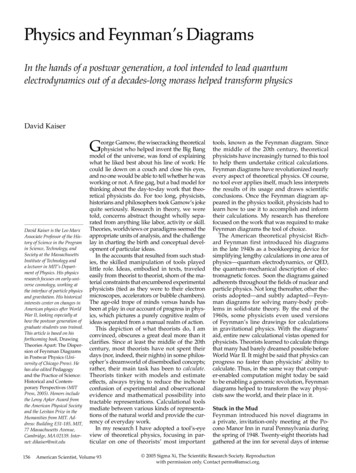
Figure 7. After World War II, the scale of equipment used by high-energy physicistsin the United States grew enormously. Here, E. O. Lawrence and his staff pose withthe newly renovated 184-inch synchrocyclotron at the Berkeley Radiation Laboratory,1946. Such particle accelerators attracted large teams of experimental physicists, whoquickly found themselves keepers of a “zoo” of unanticipated new particles. Studying the behavior of these nuclear particles became the order of the day. (Photographcourtesy of Lawrence Berkeley National Laboratory.)Building on the topology of the diagrams, Dyson generalized from these worked examplesto offer a proof that problems in QED could berenormalized.More important than his published articles,Dyson converted the Institute for AdvancedStudy into a factory for Feynman diagrams. Tounderstand how, we must first step back andconsider changes in physicists’ postdoctoraltraining during this period. Before World WarII, only a small portion of physicists who completed Ph.D.’s within the United States went onfor postdoctoral training; it was still commonto take a job with either industry or academiadirectly from one’s Ph.D. In the case of theoretical physicists—still a small minority amongphysicists within the U.S. before the war—thoseFigure 8. Faced with the influx of new and unexpected particles and interactions,some theoretical physicists began to use Feynman diagrams as pictures of physicalprocesses. The hope was that simple Feynman diagrams could help the physicistsclassify the new nuclear reactions, even if the physicists could no longer pursue perturbative calculations. (Reprinted from Marshak 1952.)162American Scientist, Volume 93who did pursue postdoctoral training usuallytraveled to the established European centers.It was only in Cambridge, Copenhagen, Göttingen or Zurich that these young Americantheorists could “learn the music,” in I. I. Rabi’sfamous phrase, and not just “the libretto” of research in physics. On returning, many of thesesame American physicists—among them Edwin Kemble, John Van Vleck, John Slater and J.Robert Oppenheimer, as well as Rabi—endeavored to build up domestic postdoctoral traininggrounds for young theorists.Soon after the war, one of the key centersfor young theorists to complete postdoctoral work became the Institute for AdvancedStudy, newly under Oppenheimer’s direction.Having achieved worldwide fame for his roleas director of the wartime laboratory at LosAlamos, Oppenheimer was in constant demand afterward. He left his Berkeley post in1947 to become director of the Princeton institute, in part to have a perch closer to hisnewfound consulting duties in Washington,D.C. He made it a condition of his acceptingthe position that he be allowed to increasethe numbers of young, temporary memberswithin the physics staff—that is, to turn theinstitute into a center for theoretical physicists’postdoctoral training. The institute quicklybecame a common stopping-ground for youngtheorists, who circulated through what Oppenheimer called his “intellectual hotel” fortwo-year postdoctoral stays.This focused yet i

the interface of particle physics and gravitation. His historical interests center on changes in American physics after World War II, looking especially at how the postwar generation of graduate students was trained. This article is based on his forthcoming book, Drawing Theories Apart: The Disper-sion of F