WIXLIB

2.2.2 Forex StrategiesIn this project, we examine several strategies such as Mean Reversion, Risk Premia, Carry Tradeand Momentum, and we finally found that the latter two could reap the profit in the normal timeand create a crisis alpha during the financial stress.For Forex Carry Trade strategy, it is a common practice in foreign exchange market. The strategysimply sells (shorts) the currency pair with lower interest rate and buys (longs) high-interest ratecurrency pair. Its profit is from the spread of the rates between two or several countries. Forsimplicity, it is similar to say you borrow the money from countries that require lower rate andinvest those money into other countries with higher rate. In this strategy, the parameter to bechanged is the weight in the long/short pair.For the Forex Momentum, it is a trend-following strategy. The strategy buys (longs) assets thatperform well historically and sells (shorts) the one performing poorly in the past. Since 252-daymomentum is recognized in the community (Rohrbach, Suremann & Osterrieder, 2017; Varadi,2016), we decided to follow it and find the currency pairs with top strongest 252-momentum tohold. The parameters to be tested are number of pairs with strong momentum to long and whetherwe should short the pair(s) with top lowest momentum among all currency pairs.2.2.3 Evaluation MetricsBefore introducing the two Ratios that we used as the measurement in the project, we would liketo introduce several important measures: Compound Annual Growth Rate (CAGR), AnnualizedVolatility (σ), and Max Drawdown (MDD). They are defined in the following:Notations: Denote N as number of trading days and Vt as the portflio value at day t wheret {0, 1, . . . , N }.1. CAGR: It is an annualized rate of return for an investment to grow in T year(s). We assumethat there are 252 trading days per year, so we can simply divide the number of trading daysby 252 to get T.T CAGR VNV0 TN252 12. σ: Volatility is a statistical measure of the dispersion of returns, and it is measured as thestandard deviation between returns during a period. Usually, we calculated the volatilitybased on the daily return; thus, we have to multiply the result by square root of 252 to getthe Annualized Volatility. The formula is defined as follows:PNσ R̄) · 252,N 1i 1 (Rtwhere Rt is the daily realized return on day t and R̄ is the average of all realized returns in Ndays.6

3. MDD: Drawdown (DD) is the measure of the decline from a historical peak to the currentlevel, and the Max Drawdown (MDD) on day t is the maximum observed loss from a peakto a trough of a portfolio from day 0 to day t. They are defined by:DDt Vt 1, where t {0, . . . , N }max{V0 , . . . , Vt }Figure 1: Equity Curve ExampleFigure 2: Illustration of Drawdown Corresponding to the Equity Curve Example7

M DDt min{DD0 , . . . , DDt }, where t {0, . . . , N }Figure 3: Drawdown Diagram ExampleFigure 4: Illustration of Max Drawdown Corresponding to the Drawdown Diagram ExampleAs marked in the Drawdown Diagram Example, it is obvious to note that the Max Drawdownreachs to a new level once a new valley is achieved.8

In the project, we aim to find a portfolio that is profitable with acceptable risk. Thus, we evaluatedthe performance of a portfolio by profitability and some risk-adjusted measures such as SharpeRatio and MAR Ratio.For the Sharpe Ratio, we used the average of 6-Month rolling Sharpe Ratio instead of the SharpeRatio over the whole trading period. The definition of Sharpe Ratio is:Sharpe Ratio CAGR Rf,σwhere Rf is the annual risk-free rate.Figure 5: Illustration of 6-Month Rolling Sharpe Ratio and the Ratio for the PortfolioFor the MAR Ratio, it is a measure that describe the frequency of the portfolio to recover fromthe most significant drawdown. For example, if the MAR ratio is 0.5, it means that the annualgrowth rate is 0.5 times of your Max Drawdown. That is, it might require 2 years for the portfolioto recover averagely. It is defined as follows:MAR Ratio 9CAGRM DD

3 Backtesting ResultsDuring the backtest, we set the original capital as 10 Million USD to ensure that the liquidityissue has not been overlooked in the test. Furthermore, the testing period of the backtesting resultsis from 1st January 2005 to 30th April 2020 for the following reasons:1. The forex data from OANDA Brokerage Forex Data is available since 2004 and the ForexMomentum strategy requires 1-year warm-up period after the data is available for generatingthe signal from 252-day momentum.2. The gold ETF (GLD) in the Permanent Portfolio is incepted after the mid-November in2004, and other 3 components are incepted earlier than GLD.3. Since we would like to set our currencies universe as big as possible to prevent losing theprofitable opportunities from some currencies, several currency pairs whose data is availablesince February 2007, such as Turkish Lira (TRY), are included into the strategies since 2007.Be reminded that we did not select Onshore Chinese Yuan (CNY) into our universe eventhough its price data is also available from February 2007.4. As the economy of China is currently ranked the second in the world, keeping ChineseRenminbi (CNY for onshore/CNH for offshore) in our universe to be a good counterpart ofUSD in our forex strategies sounds logical. However, we decided to delete it from our universefor two reasons: First, the onshore Chinese Yuan (CNY) is not tradable outside mainlandChina and the exchange rate is controlled by the central bank, so the final backtest resultwould rather be theoretical than a practical investment strategy if we included it into ouruniverse as a possible asset to hold. This contradicts to our goal that we wish to propose anidea to enhance Permanent Portfolio in practice. Second, despite the fact that the exchangerate of the offshore Chinese Yuan (CNH) is freely determined by the market, its data is onlyavailable since August 2015, which might not be a suitable choice to be included.5. We believe that testing whether the portfolio can survive during crises is an important partof algo trading. Thus, we deliberately include Global Financial Crisis in 2007-2008 and 2020Stock Crash from Mid-February to Mid-March in 2020 in our testing period.10

3.1 Forex Carry Trade (FCT)In this strategy, we extracted the central bank interest rate from Quandl. For the trading universe,there are only 9 currencies whose rate is available on Quandl and we finally picked 7 out of these 9currencies since India Rupee (INR) and Chinese Renminbi (CNY) are not in our tradable universe.We only rebalanced monthly to adjust our positions provided that the interest rate fluctuationsare expected to be rare within a month and it will be costly for us to rebalance our position withhigher frequency.3.1.1 Important terminologiesBefore explaining how we decided the weight and number of pairs to long and short, we wouldlike to introduce several terms for a better understanding of this kid of long-short strategy. Inthis strategy, we can divide our positions into three parts: (1) U.S. Dollar, (2) Long position inthe currency, and (3) Short position in the currency. We denote their values as Cash, Value ofLong Position (VLP) and Value of Short Position (VSP) respectively. Note that VSP usually is anegative number. Then we define Total Equity (TE), Dollar Net Exposure (DNE), Gross Exposure(GE), Percent Net Exposure (%NE), and Percent Gross Exposure (%GE) in the following:T E Cash V LP V SP DN E V LP V SP GE V LP V SP DN E%N E TEGE%GE TE11

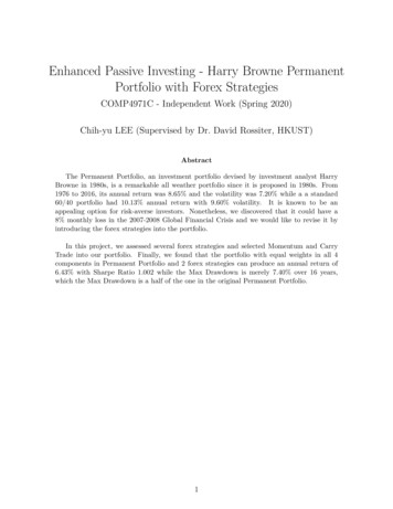
3.1.2 Weight in the currency pairsTaking into account that changing the weight in the currency pairs is similar to leverage, in thissection, we only compare three cases : %GE 100%, %GE 150%, and %GE 200%. Firstof all, it makes no sense for us to set %GE 100% under the stipulation that the strategy itselfwould be incorporated into our portfolio as a component and there would be some idle cash if wedid not set the %GE at least 100%. Moreover, we believe that it is not proper to have more than100% exposure in either the long or short position, i.e. %GE 200%, even though the Dollar NetExposure (DNE) is 0 for our Carry Trade. Finally, besides selecting the cases that %GE 100%and %GE 200%, we also select %GE 150% as a midpoint in between of 100% and 200%.Case I: 100% Gross ExposureFigure 6: Equity Curve for FCT with 100% GEFigure 7: Annual Return Diagram for FCT with 100% GEWe can observe that the payoff of the FCT strategy with GE 100% is much less attractive thaninvesting in SPY alone from the equity curve. Nevertheless, it is easy to point out a signficantgrowth of 22% in 2008, and it will be a beneficial component for us to survive during the recessions.Its annual return is merely 2.69% while the Max Drawdown is 16.9%. Overall, its profitability isnot desirable and will harm our profits considerably with its low return.12

Case II: 150% Gross ExposureFigure 8: Equity Curve for FCT with 150% GEFigure 9: Annual Return Diagram for FCT with 150% GESimilar to the one with 100% GE, the strategy with 150% GE is less attractive than investing inSPY. It produced an around 4% annual return over 16 years and more than 30% annual return in2008. Yet, it is not the optimal one for us to consider it as the final strategy since our goal is tofind a way to hedge the risk while not to sacrifice too much.13

Case III: 200% Gross ExposureFigure 10: Equity Curve for FCT with 200% GEFigure 11: Annual Return Diagram for FCT with 200% GECompared to two cases discussed in this section, it is more desirable for us to have 200% GE asthe final strategy for two reasons. First, the annual returns from both cases with 100% and 150%GE are not sufficient to maintain the profitability of the original Permanent Portfolio, which theannual return of Permanent Portfolio is above 7%. Second, we require the strategy to have a highcrisis alpha for conpensating the possible losses in the Permanent Portfolio during the crises. Itwill be acceptable for us to invest a small portion of our capital to the strategy with a 32.4% MaxDrawdown while having an annual return of 45% in 2008 and an annualized return of 27% in 2020.After making comparisons for three parameters in this strategy, we finally obtained an optimal1Forex Carry Trade strategy with annual return of 5.36%, Sharpe Ratio 0.346, and MAR Ratio 0.165with %GE 200%. Although these numbers alone are not attractive, we are confident that itscrisis alphas and long-term positive profitability can help us enhance the Permanent Portfolio as ahedge during the crisis. Next, we continue our evaluation on another strategy - Forex Momentum.1After some investigations, we explore that the performance can be further improved if we long/short more pairs.For details, please refer to Appendix A14

3.2 Forex Momentum (MOM)In the strategy, we investigate the best parameters that can effectively reap profits while createcrisis alphas to hedge against the downside of the original Permanent Portfolio. We consider thestrength of 252-day momentum as the signal for us to decide which currency pair to trade. Recallthat the parameters to be researched on are number of currencies to long and whether we shouldshort currencies with low momentum.3.2.1 Number of currencies with strong momentum to longIn light of the fact that there are 18 currencies in our forex universe, we decided to examine theperformance of longing 1 to 9 currencies. The following is the summary table for 9 long-only cases:Table 1: Summary of All 9 Long-Only StrategiesRank123456789# To 00.1900.1670.1850.143Sharpe 90.012-0.008MAR Rank123457689Total Rank33771013141518In the above table, we found that the strategies that long either 1 or 2 currencies with strongestmomentum are the front runners among these 9 choices. Other than these two strategies, thereare no strategies that can provide us a Sharpe Ratio of higher than 0.25 nor more than 0.1 MARRatio. Further, we notice that longing 2 pairs is the best in terms of Sharpe Ratio while longing1 pair is the best for MAR Ratio. Next, we will discuss their profitability and equity curves indetails.15

Case I: Long the currency with the strongest momentumFigure 12: Equity Curve for MOM with Longing 1 CurrencyFigure 13: Annual Return Diagram for MOM with Longing 1 CurrencyFrom the images, we note that its equity curve is not smooth due to a 9% loss in 2017. On topof that, it has some desirable crisis alphas, e.g., about 20% growth in 2008 and positive return inthe first 4 months of this year. However, its overall return of 3.58% is merely a half of the originalPermanent Portfolio and we may wish to have a strategy with a better profitability. Then, weconsider the strategy longing 2 pairs.16

Case II: Long the currencies with top 2 strongest momentumFigure 14: Equity Curve for MOM with Longing 2 CurrenciesFigure 15: Annual Return Diagram for MOM with Longing 2 CurrenciesAs shown in the images, it has a tremendous return of over 40% in 2008 and especially a 27.3%monthly return in the worst month of the original Permanent Portfolio. Apart from having ahigher crisis alpha in 2008, it also possessed a higher long-term profitability of 4.34%. Finally, wedecided to long the currencies with top 2 strongest momentum for the following reasons:1. It has a higher annual growth rate of 4.34% compared to the one of longing 1 currency. Asmentioned previously, reaping sufficient profit is also a crucial criterion for us to select aproper component in the portfolio.2. It has higher crisis alphas in 2008 and 2020 than its counterpart, which can hedge againstthe downside of the orginal Permanent Portfolio.17

3.2.2 Possibility of short currencies with top lowest momentumNext, we explore whether shorting the currencies with low momentum can boost the profits. Forsimplicity, we consider 9 cases where we long and short equal number of currencies. Similarly, thefollowing is the summary table for 9 long-short cases:Table 2: Summary of All 9 Long-Short StrategiesRank123456789# To 1620.1330.1480.0790.1030.1090.125Sharpe -0.061-0.072-0.075MAR Rank123456789Total Rank3369915151515Surprisingly, 7 out of 9 choices made us suffer from loss over the past 16 years and returns of theremaining 2 choices are not satisfactory compared to the strategy that only longs 2 currency pairswith the highest momentum. Therefore, we decide not to short the currency pair(s) with weakmomentum.18

3.3 Evaluation of the weight for 4 components and 2 strategiesAfter selecting proper parameters for 2 strategies above, we would like to investigate on how wecould optimally allocate the capital to each of the components or strategies. We consider 63 caseswhere we only decide whether we would like to allocate the capital into this component or strategy.The following is the summary table for the top 10 portfolios ranked by the sum of the rank inSharpe Ratio and MAR ratio2 .Table 3: Summary of Top 10 PortfoliosRank SPY TLT GLD SHY FCT MOM CAGR MDDSharpe Sharpe Rank MAR MAR RankTotal Rank1 0%0%0%100% 0%0%2.18% 2.20%1.3541 0.989122 17% 17% 17% 17%17% 17%6.43% 7.40%1.0024 0.869263 20% 20% 20% 20%0%20%6.54% 8.20%0.9825 0.797494 20% 20% 20% 0%20% 20%7.29% 8.80%0.9657 0.8293105 25% 25% 0%25%25% 0%6.42% 9.40%1.0093 0.68310136 25% 25% 0%25%0%25%5.62% 7.30%0.9519 0.7705147 20% 20% 20% 20%20% 0%7.16% 11.00%1.0142 0.65112148 20% 20% 0%20%20% 20%5.67% 7.50%0.92611 0.7566179 25% 25% 25% 0%0%25%7.63% 10.70%0.93310 0.71381810 25% 25% 25% 0%25% 0%8.42% 13.60%0.9756 0.6191521aIf a portfolio ties with another one in Total Rank, the final rank is determined by the MAR Rank given that the Sharpe Ratios are allabove 0.9 for top 10 portfolios.As the table above shown, it is surprised that the original Permanent Portfolio is not on the top10 with the criteria given its MAR ratio is ranked the 22th among all 63 portfolios. However, it isnotable that all of them have less than 10.70% Max Drawdown, more than 0.877 Sharpe Ratio andat least 0.683 MAR Ratio over 16-year backtesting period, which the Sharpe Ratio for the wellknown investor Warren Buffett is around 0.8 (Frazzini, Kabiller & Pedersen, 2018). Especially, theportfolio that allocates all the capital in short-term U.S. Treasury Bills (SHY) gave us the highestSharpe Ratio of 1.354 and the highest MAR ratio of 0.989. Nevertheless, it seems not desirable forus to receive around 2.2% gain annually in return since holding 100% in SHY is similar to savingyour capital into the bank deposit and earn the time value of money. After all, it is well-knownin finance that we will only earn profit through compensation for bearing risk. Next, we wouldanalyze the portfolio with 100% capital in SHY and the one with all components and strategiesequally weighted in details.2For the complete list of 63 portfolios, please refer to Appendix B19

Figure 16: Equity Curve of 100% in SHY Portfolio from Jan. 2005 to Apr. 2020Figure 17: Annual Return Diagram of 100% in SHY Portfolio from Jan. 2005 to Apr. 2020As the above figures showed, its annual returns are lower than 1% during bullish market in the2010s. The current level of the yield rate of U.S. short-term Treasury bills is 0.17%3 (“U.S.Department of Treasury”, n.d.), and it is hard to imagine that the yield rate could keep droppingfrom the current level to the negative level for a long time. Although the yield on short-termTreasury bills has dropped to negative 0.053% in March (Cox, 2020), it is nearly impossible for theU.S. Treasury Bills and Bonds, the asset class that global investors allocate their money in, to havethe negative rates for a long time. Thus, it is almost sure that the yield rate of the Short-TermBills will climb to a higher level so that the price of SHY will drop and the profit of holding SHYwill be significantly affected accordingly. We can conclude that it is still highly possible for theinvestors of SHY to receive 1% annual returns or even less in the future given that the bond priceis inversely correlated to its yield rate, which is known as risk-free rate for investors. In conclusion,it is absolutely not a good idea for investors to invest all their money in SHY.3As of 26th May, 202020

Then, we consider the portfolio with equal weights in all 4 Permanent Portfolio components and2 forex strategies. It generated 6.43% of CAGR while leading to only 7.40% of Max Drawdown.Moreover, its Sharpe Ratio is 1.002 and MAR Ratio is 0.869, which is ranked the 4th and 2ndamong all the 63 portfolios respectively.Figure 18: Equity Curve of the Equal Weighted Portfolio from Jan. 2005 to Apr. 2020Figure 19: Annual Return Diagram of the Equal Weighted Portfolio from Jan. 2005 to Apr. 2020As shown in the above figures, the portfolio has a similar payoff to the one that buys and holds theSPY in Feburary 2020, the trough of the current crisis, while the portfolio has a much stable andless volatile equity curve. Moreover, there is only one negative return in a year over 16-year tradingperiod, which the annual loss in 2013 is merely 3%. Surprisingly, the portfolio has significant cris

The Permanent Portfolio, an investment portfolio devised by investment analyst Harry Browne in 1980s, is a remarkable all weather portfolio since it is proposed in 1980s. From 1976 to 2016, its annual return