Transcription
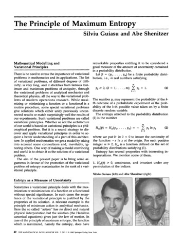
The Principle of Maximum EntropySilviu Guiasu and Abe ShenitzerMathematical M o d e l l i n g andVariational PrinciplesThere is no need to stress the importance of variationalproblems in mathematics and its applications. The listof variational problems, of different degrees of difficulty, is very long, and it stretches from famous minimum and maximum problems of antiquity, throughthe variational problems of analytical mechanics andtheoretical physics, all the w a y to the variational problems of m o d e r n operations research. While maximizing or minimizing a function or a functional is aroutine procedure, some special variational problemsgive solutions which either unify previously unconnected results or match surprisingly well the results ofour experiments. Such variational problems are calledvariational principles. Whether or not the architectureof our world is based on variational principles is a philosophical problem. But it is a sound strategy to discover and apply variational principles in order to acquire a better understanding of a part of this architecture. In applied mathematics we get a model by takinginto account some connections and, inevitably, ignoring others. One w a y of making a model convincingand useful is to obtain it as the solution of a variationalproblem.The aim of the present paper is to bring some arguments in favour of the promotion of the variationalproblem of entropy maximization to the rank of a variational principle.remarkable properties entitling it to be considered agood measure of the amount of uncertainty containedin a probability distribution.Pm) be a finite probability distriLet p (Pl . . . . .bution, i.e., rn real numbers satisfyingPk 0, (k 1 . . . . .m); Pk 1.k lThe number Pk may represent the probability of the kth outcome of a probabilisfic experiment or the probability of the k-th possible value taken on by a finitediscrete random variable.The entropy attached to the probability distribution(1) is the numbermHm(p) Hm(pl . . . . .Pm) Pk In Pk- -(2)k lwhere we put 0 9 In 0 0 to insure the continuity ofthe function - x In x at the origin. For each positiveinteger m i 2, H m is a function defined on the set ofprobability distributions satisfying (1).Entropy has several properties with interesting interpretations. We mention some of them.1. Hm(p) O, continuous, and invariant under anypermutation of the indices.Silviu Guiasu (left) and Abe Shenitzer (right)Entropy as a Measure of UncertaintySometimes a variational principle deals with the maximization or minimization of a function or a functionalwithout special significance. In such cases the acceptance of the variational principle is justified by theproperties of its solution. A relevant example is theprinciple of minimum action in analytical mechanics.Here the so called "action" has no direct and naturalphysical interpretation but the solution (the Hamiltoncanonical equations) gives just the law of motion. Incase of the principle of maximum entropy, the functionwhich is maximized, namely the entropy, does have42(1)THE MATHEMATICAL INTELLIGENCER VOL. 7, NO. 1 9 1985 Springer-Verlag New York
possible outcome (that is, a strictly deterministic experiment) contains no u n c e r t a i n t y at all; we k n o wwhat will happen before performing the experiment.This is just property 2. If to the possible outcomes of3. Hm(Pl . . . . .Pro) Hm I(Pl . . . . .Pro, 0).a probabilistic experiment we a d d another outcome4. Hm(pi . . . . .Pm) Hm(1/rn . . . . .1/rn), with equality having the probability zero, the amount of uncertaintywith respect to what will happen in the experimentif and only if Pk l / m , (k 1 . . . . .rn).remains unchanged (property 3). Property 4 tells us5. If ('rh, 1. . . . . rm,n)'is a joint probability distri- that in the class of all probabilistic experiments havingbution whose marginal probability distributions are p m possible outcomes, the maximum uncertainty is con (Pl . . . . .Pro) and (ql . . . . .q,), respectively, tained in the special probabilistic experiment whoseoutcomes are equally likely. Before interpreting thethenlast two properties let us consider two discrete randomvariables X and Y, whose ranges contain rn and n nuHmn( rl,1 . . . . . rm,n) Hm(pl . . . ., P ) merical values, respectively. Using the same notationsmPk Hn (Wk,1/Pk, " 9 9 , Wk,n/Pk)(3) as in property 5, suppose that is the joint probabilitydistribution of the pair (X, Y), and p and / are thek lmarginal probability distributions of X and Y, respecwhere the conditional entropy Hn('rtk,1/Pk . . . . .";rk,n/Pk) tively. In this case equality (3) may be written moreis c o m p u t e d only for those values of k for which compactlypk#O.H(X, Y) H(X) H(YIX )(5)6. With the notations given abovewhere2. If p has only one component which is different fromzero (i.e., equal to 1) then Hm(P) O.mk lPk H,,('rrk, I/Pk. . . . ."n*,,,/Pk) H,(ql . . . . .q,,)H ( X . Y ) Hmd rl,X . . . . .(4)H(X) Hm(Pl . . . . 'm,.), Pm)and wherewith equality if and only ifm"rrkA Pk qr (k 1 . . . . .m; ! 1 , . . . ,n),H ( Y [ X ) , Pk Hn( k,1/Pk . . . . . k,n/Pk)k lin which case (3) becomesH m , ( ) H,,(p) Hn(-q).All these properties can be proved in an elementarymanner. Without entering into the technical details,we note that properties 1 - 3 are obvious while property 5 can be obtained by a straightforward computation taking into account only the definition of entropy. Finally, from Jensen's inequalityis the conditional entropy of Y given X. According to(5), the amount of uncertainty contained in a pair ofrandom variables (or, equivalently, in a c o m p o u n d - or product--probabilistic experiment) is obtained bysumming the amount of uncertainty contained in onecomponent (say X) and the uncertainty contained inthe other component (Y) conditioned by the first one(X). Similarly, we get for H ( X , Y ) the decompositionH(X, Y) H(Y) H(XIY )(6)where,ak f(bk) f ( k lak bk )k lapplied to the concave function f(x) - x In x, weobtain property 4 by putting a k l / m , b k Pk, k 1. . . . . m, and the inequality (4) by putting a k Pk, bk k,t /Pk, k 1 . . . . .m, for any 1 . . . . .n, and,in the last case, summing the resulting n inequalities.Interpretation of the above properties agrees withcommon sense, intuition, and the reasonable requirements that can be asked of a measure of uncertainty.Indeed, a probabilistic experiment which has only oneH ( Y ) Hn(q . . . . .qn)andH(XIY) q t H m \ q'.- -qt / " IHereHm( l,dqt . . . . . rm,t/qt)THE MATHEMATICAL INTELLIGENCER VOL. 7, NO. 1, 198543
is the conditional entropy of X given the [ -th value ofYt. Hm is defined only for those values of for whichqr 0. From (5) and (6) we getH(X) - H(X[Y) H(Y) - H(YIX )which is the so-called "uncertainty balance", the onlyconservation law for entropy.Finally, property 6 shows that some data on X canonly decrease the uncertainty on Y, namelyH(YIX ) H ( Y )(7)with equality if and only if X and Y are independent.From (5) and (7) we getH(X, Y) H(X) H(Y)with equality if and only if X andFortunately this inequality holdscomponents. More generally, forwith arbitrary finite range we canH(X 1. . . . .ms) H(X,) . . .Y are independent.for any number ofs random variableswrite H(Xs)with equality if and only if X 1. . . . .independent. ThereforeW ( X 1. . . . .Xs) H(Xi)-Discrete entropy as a measure of uncertainty whsintroduced by C. E. S h a n n o n [12] by analogy withBoltzmann's H function [1] in statistical mechanics. Itwas also used by Shannon as a measure of information, considering information as removed uncertainty.Before a probabilistic experiment is performed the entropy measures the amount of uncertainty associatedwith the possible outcomes. After the experiment thee n t r o p y measures the a m o u n t of supplied information. We stress that this is the first time a mathematicalfunction has aimed to measure the uncertainty contained in a probabilistic e x p e r i m e n t - - a n entity so different from measurable characteristics of the real worldsuch as length, area, volume, temperature, pressure,mass, charge, etc.Is the Shannon entropy unique? The answer depends on what properties are taken as the axioms forthe measure of uncertainty. Khintchine [9] proved thatproperties 1, 3, 4, and 5, taken as axioms (which isquite reasonable from an intuitive point of view),imply uniquely the expression (2) for the measure ofuncertainty up to an arbitrary positive multiplicativeconstant. This allows us to choose arbitrarily a basegreater than 1 for the logarithm without affecting thebasic properties of the measure.X s are globallyH ( X 1. . . . .Xs) 0The Principle of Maximum Entropyi 1measures the global dependence b e t w e e n the randomvariables X 1. . . . .X s, that is, the extent to which thesystem (X 1. . . . .Xs), due to i n t e r d e p e n d e n c e ,makes up "something more" than the mere juxtaposition of its components. In particular, W 0 if andonly if X 1. . . . .X s are independent.Note that the difference between the amount of uncertainty contained by the pair (X, Y) and the amountof d e p e n d e n c e b e t w e e n the c o m p o n e n t s X and Y,namely,d(X, Y) H(X, Y ) - W(X, Y)or, equivalently,d(X, Y) 2H(X, Y ) - H(X) - H(Y) H(XIY ) H(YIX ),is a distance between the random variables X and Y,with the two random variables considered identical ifeither one c o m p l e t e l y determines the other, or ifH(X]Y) 0 and H(YIX ) 0. Therefore, the "purerandomness" contained in the pair (X, Y), i.e., theuncertainty of the whole, minus the dependence between the components, measured by d(X, Y), is a distance. This geometrizes chaos!44THE MATHEMATICAL 1NTELLIGENCER VOL, 7, NO. 1, 1985Let us go back to property 4: The uncertainty is maximum when the outcomes are equally likely. The uniform distribution maximizes the entropy; the uniformdistribution contains the largest a m o u n t of uncertainty. But this is just Laplace's Principle of InsufficientReason, according to which if there is no reason todiscriminate between two or several events the beststrategy is to consider t h e m as equally likely. Ofcourse, for Laplace this was a subjective point of view,based on prudence and on common sense. Indeed,without knowing anything about entropy we applyLaplace's Principle of Insufficient Reason in everydaylife, even in analyzing the simplest experiments. Indeed, in tossing a coin we usually attach equal probabilities to the two possible outcomes not after a longseries of repetitions of this simple experiment followedby a careful analysis of the stability of the relative frequencies of the possible outcomes but simply becausewe apply Laplace's Principle and realize that we haveno good reasons for discriminating between the twooutcomes. But, as we have already seen, if we acceptthe Shannon entropy as the measure of uncertainty,then property 4 is just the mathematical justificationof the Principle of Maximum Entropy, which assertsthat entropy is maximized by the uniform distributionw h e n no constraint is imposed on the probability distribution. In such a case, our intuition, based on our
past experience, gives us the right solution. But w h a th a p p e n s w h e n there are some constraints imposed onthe probability distribution?Before answering this question let us see w h a t kindsof constraints m a y be imposed. Quite often in applications we have at our disposal one or several meanvalues of one or several r a n d o m variables. Thus instatistical mechanics the state functions are r a n d o mvariables because the state space is a probability spaceand we can m e a s u r e only some m e a n values of suchstate functions. For instance, to each microscopic statethere corresponds a well-defined value of the energyof the system. But we cannot determine w i t h certaintythe real, unique, microscopic state of the system atsome instant t, a n d so we construct instead a probability distribution on the possible states of the system.Then the energy becomes a r a n d o m variable and w h a twe can really measure, at the macroscopic level, is them e a n value of this r a n d o m variable, i.e., the macroscopic energy. The macroscopic level is the level ofm e a n values a n d some of these m e a n values can bemeasured. But we n e e d a probabilisfic model of themicroscopic level, i.e., a probability distribution on thepossible microscopic states of the system. In general,there are m a n y probability distributions (even an infinity!) c o m p a t i b l e w i t h the k n o w n m e a n values.Hence the question: W h a t probability distribution is"best" and with respect to w h a t criterion?In 1957 E. T. Jaynes [8] gave a very natural criterionof choice by introducing the Principle of M a x i m u m Entropy: From the set of all probability distributions compatible with one or several m e a n values of one or several r a n d o m variables, choose the one that maximizesShannon's entropy. Such a probability distribution isthe "largest one"; it will ignore no possibility, beingthe most uniform one, subject to the given constraints.I n t r o d u c e d for solving a p r o b l e m in statistical mechanics, the Principle of Maximum Entropy has become a widely applied tool for constructing the probability distribution in statistical inference, in decisiont h e o r y , in p a t t e r n - r e c o g n i t i o n , in c o m m u n i c a t i o ntheory, and in time-series analysis, because in all theseareas what we generally k n o w is expressed by m e a nvalues of some r a n d o m variables and w h a t we need isa probability distribution which ignores no possibilitysubject to the relevant constraints.To see h o w this principle works let us take the simplest possible case, the case in which we k n o w them e a n value E(f) of a r a n d o m variable f w h o s e possiblevalues are h . . . . .fm" We need a probability distribution p (Pl . . . . .Pm), 1. . . . .m); k lsatisfying the constraint(9) Pk"k lIn the trivial case m 2, the m e a n value E(f) uniquelyd e f i n e s the c o r r e s p o n d i n g p r o b a b i l i t y d i s t r i b u t i o nfrom the linear equationEft) flPl f2(1 - Pl).But for a n y m I 3 there is an infinity of probabilitydistributions (8) satisfying (9). Applying the Principleof M a x i m u m Entropy we choose the most uncertainprobability distribution, i.e., the probability distribution that maximizes the e n t r o p ymHm(p) - pk ln pkk lsubject to the constraints (8) a n d (9). Of course, H m isa c o n c a v e a n d c o n t i n u o u s f u n c t i o n d e f i n e d in theconvex d o m a i n characterized by (8) and (9). There isonly one global m a x i m u m point belonging to the o p e nset{P (P . . . . .Pm)lPk O, k 1 . . . . .Pk -- 1 O,k lfkPk--m;E f t ) 0}.k lTaking the Lagrange functionL Hm(Pl . . . . .Pm) - o Pk -- 1w h e r e x a n d 13 are the L a g r a n g e multipliers corresponding to the two constraints, and putting the firstorder partial derivatives equal to zero we getaL3pk-In Pk -- 1 -- ot -- fk O, ( k 1 .m),m3L10OL , PkO,k lm3LOf3Eft) - , fk Pkk lO.Thus the solution ismPk 0 , ( kmE(f) Pk 1(8)Pk --e - 0f m, (k 1. . . . .m)(10)Y', e-"J,r lTHE MATHEMATICAL INTELLIGENCER VOL. 7, NO. 1, 1985 45
where 130 is the solution of the exponential equationm[fk -- E(f)] e-f (f -E(f)) 0.(11)k lIf the random variable f is nondegenerate (i.e., iff takeson at least two different values), such a solution existsand is unique because the functionmG(f3) , Ilk -- E(f)] e- (f -E(f))(12)of the Principle of M a x i m u m Entropy is Pl 0.1035103, P2 0.2103835, P3 0.6861062. This is themost uniform probability distribution compatible withthe given mean value. For some other constraints, theexact values of the Lagrange multipliers introduced formaximizing the entropy may be determined exactly.Without entering into technical details we mentionsome remarkable results relating to the Principle ofMaximum Entropy:a) If f is a random variable whose range is countable,namely, ifk l{kulu 0, k 0,1,2 . . . . }is strictly decreasing withlim13 - - G(6) ,limG( ) - oo.6--* We have already seen that when there is no constraint, the solution of the Principle of Maximum Entropy is the uniform probability distribution. When themean value E(f) of a random variable f is given, thenthe solution of the Principle of Maximum Entropy is(10) or, equivalently,1- ep k -- - ,v( )- Jk, (k 1 . . . . .(this is true of the energy in quantum mechanics--inwhich case u is the quantum of e n e r g y - - o r of manydiscrete functions in operations r e s e a r c h - - i n whichcase u is the unit), and if the mean value E(f) is given,then the probability distributionPk O, (k 0,1 . . . .k Omaximizing the countable entropy:m)whereH -mk land 60 is the unique solution of the equationd In cI (6)-E(f).This is just the Gibbs, or canonical, distribution encountered in almost all books on statistical mechanicsand, more recently, in some books on decision theory.Now we see w h y the canonical distribution is usefulin applications: It is the most uncertain one, the mostuniform one, it ignores no possibility subject to theconstraint given by the mean value E(f).Since (11) is an exponential equation, its solution 60may be a transcendental number. However, the factthat the function G given by (12) is strictly decreasingpermits us to approximate the solution 130 with greataccuracy.For instance, let m 3, h 12, f2 15, f3 20and the mean value E(f) 18.12. Using a simple TI57 pocket calculator, we can obtain in a few minutesthe solution of equation (11) (correct to six decimals),namely, 60 - 0.2364201. The corresponding solution46Z Pk In Pkk Ois ( ) , e - fkdf ), , Pk 1THE MATHEMATICAL INTELLIGENCER VOL. 7, NO. 1, 1985Pk u(E(f)) k(u E(f)) k l" k 0,1,2 . . . . .We see that the unit u and the mean value E(f) completely determine the solution of the Principle of Maximum Entropy. The importance of this probability distribution is stressed by M. Born [2].Before discussing the continuous case, we note anunusual property of entropy that permits us to maximize it even w h e n the solution is a sequence satisfyingPk 0 , Pk 1.k 0In such a case, instead of computing the partial derivatives w i t h respect to a countable set of variables(P0,Pl . . . .a n d the Lagrange multipliers corresponding to the constraints), it is enough to take intoaccount the simple equalityt lnt (t-11) - ( t -1)2,true for any t 0, where % depending on t, is a positivenumber located somewhere between 1 and t. (This
equality is obtained from the Taylor e x p a n s i o n oft In t about 1.) Applying this equality and consideringthe constraint1 (x e"if x 0O, elsewhereocE ( f ) , kU pk 176k Owe have, for o 0, 0,H-oL " l -f3E(f) - pk ln(pk e ku) k 0- , e-"-"h(pke "ku) In (pk e ku)k Oococ , e- '-"kU(pke ku -- 1) --1 -k 0e- -"ku;k Owhich is just the well-known exponential probabilitydensity function. N o w we have a justification for theusual assumption in queueing theory that the interarrival time is exponentially distributed. Such a probability distribution is the most uncertain one, the mostprudent one, and it ignores no possibility subject tothe mean interarrival time p,.c) Of course, it is possible to have many constraints.Suppose that, in the continuous case, we know boththe m e a n p, and the variance cr2 of a c o n t i n u o u srandom variable whose probability density function issquare-integrable. The agreeable surprise is that, insuch a case, the continuous entropy (13) is maximizedjust by(x - )2here the upper b o u n d is independent of the probability distribution {Pk, k 0,1 . . . . }, and we haveequality if and only ifPk e- -f ku, k 0,1 . . . .From the first constraintoce -a-f ku 1k 0we obtaine - a 1 - e -f uand from the second constraintE ( f ) , ku(1 -e - u) e -"kuk 0we obtain the solutionu(E(f)) kPk (u E ( f ) ) k l 'k 0,1 . . . .b) In the continuous case, suppose that we knowthe mean value N- of a positive continuous randomvariable whose probability density function is squareintegrable. In such a case, the continuous entropyH(g) -f2is maximized byB(x) In g ( x ) d x(13)8(x) -1crX/ e2o ,(- 176 )which is the probability density function of the normaldistribution N( , or2). Now we see w h y this probabilitydistribution has been frequently used in the applications of statistical inference and w h y it deserves theadjective "normal"; in the infinite set of square integrable probability density functions defined on thereal line with mean and variance cr2, the normal distribution (or de Moivre-Laplace-Gauss distribution) isthe distribution that is most uncertain and that maximizes the entropy. Entropy would have had to beinvented if only to demonstrate this variational property of the normal distribution!The fact that the Principle of Maximum Entropy canbe used to obtain a unified variational treatment ofsome well-known probability distributions is just onereason for its importance. In fact, we can apply thesame strategy (i.e., maximizing the entropy) subject tomore numerous and more sophisticated constraints,such as a large number of mean values (moments oforder greater than 2) of several random variables. Thesolution of the Principle of Maximum Entropy will giveprobability distributions never met before.We conclude with some comments on what is subjective and what is objective in the use of the Principleof Maximum Entropy. As a variational problem (maximize the entropy subject to constraints expressed bymean values of some random variables) it is as objective as any other mathematical optimization problem.Accepting the probabilistic entropy as a measure ofuncertainty and interpreting the solution of the Principle of Maximum Entropy from the viewpoint of theamount of uncertainty contained is, in spite of the"naturalness" of the properties 1 - 6 above, a subjectiveTHE MATHEMATICAL INTELLIGENCER VOL. 7, NO. 1, 198547
attitude. But the fact that some important probabilitydistributions from statistical inference (exponential, canonical, uniform, and, above all, the most importantone, the normal distribution) are solutions of it enablesus to say that the use of the Principle of MaximumEntropy proves to be more than a simple convention.The Principle of Maximum Entropy has implied bothsome other entropic variational problems (the minimization of the Kullback-Leibler divergence, theminimization of the interdependence) and many newapplications (for example its recent applications intime-series analysis and the entropic algorithm for pattern-recognition which proves to have the smallestmean length); but this is another story.References1. L. Boltzmann (1896) Vorlesungen fiber Gastheorie, Leipzig: J. A. Barth.2. M. Born (1969) Atomic Physics. (8-th edition). LondonGlasgow: Blakie & Son Ltd.3. L. L. Campbell (1970) Equivalence of Gauss's principleand minimum discrimination information estimation ofprobabilities. Ann. Math. Statist., 41, 1011-1015.4. J. W. Gibbs (1902) Elementary principles in statisticalmechanics developed with especial reference to the rational foundation of thermodynamics. New Haven,Conn: Yale University Press.5. S. Guiaw (1977) Information theory with applications.New York-London-Dfisseldorf: McGraw-Hill.6. S. Guia u, T. Nguyen Ky (1982) On the mean length ofthe entropic algorithm of pattern-recognition. Journal ofCombinatorics, Information & System Sciences, 7, 203211.7. S. Guia u, R. Leblanc, C. Reischer (1982) On the principle of minimum interdependence. Journal of Information & Optimization Sciences, 3, 149-172.8. E. T. Jaynes (1957) Information theory and statistical mechanics. Phys. Rev. 106, 620-630; 108, 171-182.9. A. I. Khinchin (1957) Mathematical foundations of information theory. New York: Dover Publications.10. S. Kullback (1959) Information theory and statistics. NewYork: Wiley. London: Chapman & Hall.11. E. Parzen (1982) Maximum entropy interpretation of autoregressive spectral densities. Statistics & ProbabilityLetters 1, 7-11.I lie Cartan(Euvres Completes1984. 3 portraits. Environ 4750 pages.( E n q u a t r e volumes, non livrable s par6ment)Reli D M 2 9 5 , Paris: l ditions du Centre N a t i o n a l de la Recherche ScientifiqueISBN 3-540-13629-0The Complete Works of/ lie Cartan, originally published in 1952, were out of print for several years buthave now been reissued as a 4-volume set.l lie Cartan's work is, by virtue of its depth, its varietyand its great originality, increasingly being recognisedas a turning point in the evolutionary history of geometry, and its far-reaching consequences are not yetcompletely explored. Many contemporary geometers.still draw their inspiration from reading Cartan'swork.Many of the concepts l lie Cartan introduced havespread their impact to other areas of mathematics.The geometry of bundles, for instance, has established itself as a classical topic, especially since thedevelopment of gauge theory in theoretical physicshas made it the framework for the study of particleinteractions. The role played by transformationgroups in the understanding of geometric problemshas been confirmed. Many aspects of Riemanniangeometry have also penetrated areas such as topologyand group theory. The current interest in non-linearpde's is drawing attention back to Cartan's development of the subject.The three parts of the Complete Works correspond tothree different subject areas: I. Lie groups, II. algebra,differential systems and the equivalence problem,III. geometry and other topics. They collect togetherall his research articles, but not monographs or cdrrespondence. However they do also include a report onhis work written by l lie Cartan himself in relationwith his candidacy to the French Academy of Sciences.This new edition also features the Obituaries for t lieCartan written by S. S. Chern and C. Chevalley for theAmerican Mathematical Society, and byH. Whitehead for the Royal Society.12. C. E. Shannon (1948) A mathematical theory of communication. Bell Syst. Techn. Journal, 27, 379-423, 623656.13. S. Watanabe (1969) Knowing and guessing. New York:Wiley.Silviu GuiasuDepartment of MathematicsYork University4700 Keele StreetDownsview, Ont. M3J 1P3CanadaAbe ShenitzerDepartment of MathematicsYork University4700 Keele StreetDownsview, Ont. M3J 1P3Canada48 THE MATHEMATICALINTELLIGENCERVOL. 7, NO. 1, 1985Springer-VerlagBerlin Heidelberg NewYork TokyoTiergartenstr. 17, D-6900 Heidelberg 1, 175 Fifth Ave., NewYork, NY 10010, USA,37-3, Hongo 3-chome, Bunkyo-ku, Tokyo 113, Japan
THE MATHEMATICAL INTELLIGENCER VOL. 7, NO. 1, 1985 43 . is the conditional entropy of X given the [ -th value of Yt. Hm is defined only for those values of for which qr 0. From (5) and (6) we get H(X) - H(X[Y) H(Y) - H(YIX ) w
