WIXLIB

theory would seem to predict that the electron mass is huge, of order of the inverselength of the string, unless there is some tiny number which sits out in front of theintegral. It turns out that string theory can do more than just cut off the integral, itcan also add an additional integral which cancels off a large chunk of the first integral,leaving a more realistic result for the electron mass. This cancellation is a consequenceof “supersymmetry” which, as it turns out, is necessary in some form for string theoryto be mathematically consistent.So by working with objects of finite extent, we accomplish two things. First off, allof our integrals are finite, and in principle, if string theory were completely understood,we would only need one measurement to make predictions for gravitational interactionsat arbitrary distances. But also we gain enormous predictive power (at least in principle,its not quite so simple as we shall see). Indeed in the standard model of particle physics,which correctly describes all interactions at least to energies of order 200 GeV, thereare 23 free parameters which need to be fixed by experiment, just as the electron massdoes. String theory, however, has only one such parameter in its Lagrangian, the stringlength‡ ! Never forget that physics is a predictive science. The less descriptive and themore predictive our theory is, the better. In that sense, string theory has been a holygrail. We have a Lagrangian with one parameter which is fixed by experiment, andthen you are done. You have a theory of everything! You could in principle explainall possible physical phenomena. To say that this a a dramatic simplification would bean understatement, but in principle at least it is correct. This opens a philosophicalpandoras’ box which should be discussed late at night with friends.But wait there is more! Particle physics tells us that there a huge number of“elementary particles”. Elementary particles can be split into two categories, “matter”and “force carriers”. These names are misleading and should only be understood assounds which we utter to denote a set. The matter set is composed of six quarks u,d, s, c, b, t (up, down, strange, charm, bottom, top) while the force carriers are thephoton the “electroweak bosons”, Z, W , the graviton g and eight gluons responsiblefor the strong force. There is the also the socalled “Higgs boson” for which we onlyhave indirect evidence at this point. So, in particle physics, we have a Lagrangianwhich sums over all particle types and distinguishes between matter and force carriersin some way. This is a rather unpleasant situation. If we had a theory of everythingall the particles and forces should be unified in some way so that we could write down‡A warning, this is misleading because to describe a theory we need to know more than just theLagrangian, we also need to know the ground state, of which there can be many. Perhaps you haveheard of the “string theory landscape”? What people are referring to is the landscape of possibleground states, or equivalently “vacau”. There are people that are presently trying to enumerate theground states of string theory.–7–

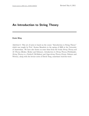
a Lagrangian for a “master entity”, and the particles mentioned would then just bedifferent manifestations of this underlying entity. This is exactly what string theorydoes! The underlying entity is the string, and different excitations of the string representdifferent particles. Furthermore, force unification is built in as well. This is clearly avery enticing scenario.With all this said, one should keep in mind that string theory is in some senseonly in its infancy, and, as such, is nowhere near answering all the questions we hopedit would, especially regarding what happens at singularities, though it has certainlyled to interesting mathematics (4-manifolds, knot theory.). It can also be said thatit has taught us much about the subject of strongly coupled quantum field theoriesvia dualities. There are those who believe that string theory in the end will eitherhave nothing to do with nature, or will never be testable, and as such will always berelegated to be mathematics or philosophy. But, it is hard not to be awed by stringtheory’s mathematical elegance. Indeed, the more one learns about its beauty the moreone falls under its spell. To some it has become almost a religion. So, as a professoronce said: “Be careful, and always remember to keep your feet on the ground lest yoube swept away by the siren that is the string”.1.2 What is String TheoryWell, the answer to this question will be givenby the entire manuscript. In the meantime, roughlyspeaking, string theory replaces point particles bystrings, which can be either open or closed (depends on the particular type of particle that is being replaced by the string), whose length, or stringlength (denoted ls ), is approximately 10 33 cm.Also, in string theory, one replaces Feynman diagrams by surfaces, and wordlines become world- Figure 1: In string theory, Feynman diagrams are replaced by sursheets.faces and worldlines are replaced byworldsheets.1.2.1 Types of String TheoriesThe first type of string theory that will be discussed in these notes is that of bosonicstring theory, where the strings correspond only to bosons. This theory, as will beshown later on, requires 26 dimensions for its spacetime.In the mid-80’s it was found that there are 5 other consistent string theories (whichinclude fermions): Type I–8–

Type II A Type II B Heterotic SO(32) Heterotic E8 E8 .All of these theories use supersymmetry, which is a symmetry that relates elementaryparticles of one type of spin to another particle that differs by a half unit of spin.These two partners are called superpartners. Thus, for every boson there exists itssuperpartner fermion and vice versa.For these string theories to be physically consistent they require 10 dimensions forspacetime. However, our world, as we believe, is only 4 dimensional and so one is forcedto assume that these extra 6 dimensions are extremely small. Even though these extradimensions are small we still must consider that they can affect the interactions thatare taking place.It turns out that one can show, non-perturbatively, that all 5 theories are part ofthe same theory, related to each other through dualities.Finally, note that each of these theories can be extended to D dimensional objects,called D-branes. Note here that D 10 because it would make no sense to speak of a15 dimensional object living in a 10 dimensional spacetime.1.3 Outline of the ManuscriptWe begin we a discussion of the bosonic string theory. Although this type of stringtheory is not very realistic, one can still get a solid grasp for the type of analysisthat goes on in string theory. After we have defined the bosonic string action, orPolyakov action, we will then proceed to construct invariants, or symmetries, for thisaction. Using Noether’s theorem we will then find the conserved quantities of the theory,namely the stress energy tensor and Hamiltonian. We then quantize the bosonic stringin the usual canonical fashion and calculate its mass spectrum. This, as will be shown,leads to inconsistencies with quantum physics since the mass spectrum of the bosonicstring harbors ghost states - states with negative norm. However, the good news isthat we can remove these ghost states at the cost of fixing the spacetime, in which thestring propagates, dimension at 26. We then proceed to quantize the string theory ina different way known as light-cone gauge quantization.The next stop in the tour is conformal field theory. We begin with an overviewof the conformal group in d dimensions and then quickly restrict to the case of d 2.Then conformal field theories are defined and we look at the simplifications come with–9–

a theory that is invariant under conformal transformations. This leads us directlyinto radial quantization and the notion of an operator product expansion (OPE) of twooperators. We end the discussion of conformal field theories by showing how the charges(or generators) of the conformal symmetry are isomorphic to the Virasor algebra. Withthis we are done with the standard introduction to string theory and in the remainingchapters we cover developements.The developements include scattering theory, BRST quantization and BRST cohomology theory along with RNS superstring theories, dualities and D-branes, effectiveactions and M-theory and then finally matrix theory.– 10 –

2. The Bosonic String ActionA string is a special case of a p-brane, where a p-brane is a p dimensional object movingthrough a D (D p) dimensional spacetime. For example: a 0-brane is a point particle, a 1-brane is a string, a 2-brane is a membrane .Before looking at strings, let’s review the classical theory of 0-branes, i.e. pointparticles.2.1 Classical Action for Point ParticlesIn classical physics, the evolution of a theory is described by its field equations. Supposewe have a non-relativistic point particle, then the field equations for X(t), i.e. Newton’slaw mẌ(t) V (X(t))/ X(t), follow from extremizing the action, which is given byZS dtL,(2.1)where L T V 12 mẊ(t)2 V (X(t)). We have, by setting the variation of S withrespect of the field X(t) equal to zero,0 δSZZ1 V m dt (2Ẋ)δ Ẋ dtδX2 XZZ V m dtẌδX boundary terms dtδX {z} X Ztake 0 VδX ,dt mẌ Xwhere in the third line we integrated the first term by parts. Since this must hold forall δX, we have that V (X(t)),(2.2)mẌ(t) X(t)which are the equations of motion (or field equations) for the field X(t). These equations describe the path taken by a point particle as it moves through Galilean spacetime(remember non-relativistic). Now we will generalize this to include relativistic pointparticles.– 11 –

2.2 Classical Action for Relativistic Point ParticlesFor a relativistic point particle moving through a D dimensional spacetime, the classicalmotion is given by geodesics on the spacetime (since here we are no longer assuminga Euclidean spacetime and therefore we must generalize the notion of a straight linepath). The relativistic action is given by the integral of the infinitesimal invariantlength, ds, of the particle’s path, i.e.ZS0 α ds,(2.3)where α is a constant, and we have also chosen units in such a way that c 1.In order to find the equations that govern the geodesic taken by a relativistic particlewe, once again, set the variation of the, now relativistic, action equal to zero. Thus,the classical motion of a relativistic point particle is the path which extremizes theinvariant distance, whether it minimizes or maximizes ds depends on how one choosesto parametrize the path.Now, in order for S0 to be dimensionless, we must have that α has units of Length 1which means, in our chosen units, that α is proportional to the mass of the particleand we can, without loss of generality, take this constant of proportionality to be unity.Also, we choose to parameterize the path taken by a particle in such a way that theinvariant distance, ds, is given byds2 gµν (X)dX µ dX ν ,(2.4)where the metric gµν (X), with µ, ν 0, 1, ., D 1, describes the geometry of thebackground spacetime† in which the theory is defined. The minus sign in (2.4) has beenintroduced in order to keep the integrand of the action real for timelike geodesics, i.e.particles traveling less than c 1, and thus we see that the paths followed by realisticparticles, in this parameterization, are those which maximize ds‡ . Furthermore, we will†By background spacetime, also called the target manifold of the theory, we mean the spacetime inwhich our theory is defined. So, for example, in classical physics one usually takes a Galilean spacetime,whose geometry is Euclidean (flat). While, in special relativity, the spacetime is taken to be a fourdimensional flat manifold with Minkowski metric, also called Minkowski space. In general relativity(GR) the background spacetime is taken to be a four dimensional semi-Riemannian manifold whosegeometry is determined by the field equations for the metric, Einstein’s equations, and thus, in GR thebackground geometry is not fixed as in classical mechanics and special relativity. Therefore, one saysthat GR is a background independent theory since there is no a priori choice for the geometry. Finally,note that quantum field theory is defined on a Minkowski spacetime and thus is not a backgroundindependent theory, also called a fixed background theory. This leads to problems when one tries toconstruct quantized theories of gravity, see Lee Smolin “The Trouble With Physics”.‡In this parameterization the element ds is usually called the proper time. So, we see that classicalpaths are those which maximize the proper time.– 12 –

choose our metrics, unless otherwise stated, to have signatures given by (p 1, q D 1) where, since we are dealing with non-degenerate metrics, i.e. all eigenvaluesare non-zero§ , we calculate the signature of the metric by diagonalizing it and thensimply count the number of negative eigenvalues to get the value for p and the numberof positive eigenvalues to get the value for q. So, consider the metric given by g00 (X)0000 0 g11 (X)000 gµν (X) 00g22 (X)00 , 000g33 (X)0 0000g44 (X)where gii (X) 0 for all i 0, 1, ., 3. It should be clear that this metric has signature(2, 3).If the geometry of the background spacetime is flat then the metric becomes aconstant function on this spacetime, i.e. gµν (X) cµν for all µ, ν 0, ., D 1, wherecµν are constants. In particular, if we choose the geometry of our background spacetimeto be Minkowskian then our metric can be written as 1 0 0 0 0 1 0 0 (2.5)gµν (X) 7 ηµν . 0 0 1 0 0 0 0 1This implies that, in a Minkowskian spacetime, the action becomesZ pS0 m (dX 0 )2 (dX 1 )2 (dX 2 )2 (dX 3)2 .Note that the signature of the above metric (2.5) is (1, 3).If we choose to parameterize the particle’s path X µ (τ ), also called the worldline ofthe particle, by some real parameter τ , then we can rewrite (2.4) as gµν (X)dX µ dX ν gµν (X)dX µ (τ ) dX ν (τ ) 2dτ ,dτdτ(2.6)which gives for the action,S0 mwhere Ẋ µ §dX µ (τ ).dτZdτq gµν (X)Ẋ µ Ẋ ν ,They are also smooth and symmetric but that does not concern us here.– 13 –(2.7)

An important property of the action is that it is invariant under which choice ofparameterization is made. This makes sense because the invariant length ds betweentwo points on a particle’s worldline should not depend on how the path is parameterized.Proposition 2.1 The action (2.7) remains unchanged if we replace the parameter τby another parameter τ 0 f (τ ), where f is monotonic.Proof By making a change of parameter, or reparametrization, τ 7 τ 0 f (τ ) wehave that fdτ 7 dτ 0 dτ, τand sodX µ (τ 0 )dX µ (τ 0 ) dτ 0dX µ (τ 0 ) f (τ ) .dτdτ 0 dτdτ 0 τNow, plugging τ 0 into (2.7) givesrZdX µ(τ 0 ) dX ν (τ 0 )S00 m dτ 0 gµν (X)dτ 0dτ 0rZdX µ (τ 0 ) dXµ (τ 0 ) m dτ 0dτ 0dτ 0s 2Z fdX µ dXµ f mdτ τdτ dτ τZ 1 r fdX µ (τ ) dXµ (τ ) fdτ m τ τdτdτrZdX µ (τ ) dXµ (τ ) m dτdτdτrZdX µ (τ ) dXµ (τ ) m dτ gµνdτdτ S0 .Q.E.D.Thus, one is at liberty to choose an appropriate parameterization in order to simplifythe action and thereby simplify the equations of motion which result from variation.This parameterization freedom will now be used to simplify the action given in (2.7).– 14 –

Since the square root function is a non-linear function, we would like to constructanother action which does not include a square root in its argument. Also, whatshould we do if we want to consider massless particles? According to (2.7) the action ofa massless particle is equal to zero, but does this make sense? The claim is that insteadof the original action (2.7) we can add an auxiliary field to it and thereby construct anequivalent action which is simpler in nature. So, consider the equivalent action givenbyZ 1 1 22S̃0 dτ e(τ ) Ẋ m e(τ ) ,(2.8)2where Ẋ 2 gµν Ẋ µ Ẋ ν and e(τ ) is some auxiliary field. Before showing that this actionreally is equivalent to (2.7) we will first note that this action is the simplification wewere looking for since there is no longer a square root, and the action no longer becomeszero for massless particles. Now, to see that this new action is equivalent with (2.7),first consider the variation of S̃0 with respect to the field e(τ ), Z 1 1 22δ S̃0 δdτ e Ẋ m e2Z 11dτ 2 Ẋ 2 δe m2 δe 2eZ 1δe dτ 2 Ẋ 2 m2 e2 .2eBy setting δ S̃0 0 we get the field equations for e(τ ),s2Ẋ Ẋ 2e2 2 e .mm2(2.9)Now, plugging the field equation for the auxiliary field back into the action, S̃0 , wehave ! 1/2!1/2 Z221ẊẊ S̃0 dτ 2Ẋ 2 m2 22mm12Z1 2Z dτ dτ2Ẋm2Ẋ 2 2m! 1/2! 1/2 Ẋ 2 m2Ẋ 2 Ẋ 2– 15 – !! Ẋ m22

1 2ZdτẊ 2 2m! 1/2 22Ẋ! 1/2 Ẋ 2dτ 22( Ẋ 2 ) ( 1)mZ 1/2 1 Ẋ 2dτ ( 2m) Ẋ 2 2Z 1/2 Ẋ 2 m dτ Ẋ 21 2ZZdτ ( Ẋ 2 )1/2rZdX µ dX ν m dτ gµνdτ dτ m S0 .So, if the field equations hold for e(τ ) then we have that S̃0 is equivalent to S0 .2.2.1 Reparametrization Invariance of S̃0Another nice property of S̃0 is that it is invariant under a reparametrization (diffeomorphism) of τ . To see this we first need to see how the fields X µ (τ ) and e(τ ) varyunder an infinitesimal change of parameterization τ 7 τ 0 τ ξ(τ ). Now, since thefields X µ (τ ) are scalar fields, under a change of parameter they transform according to0X µ (τ 0 ) X µ (τ ),and so, simply writing the above again,00X µ (τ 0 ) X µ (τ ξ(τ )) X µ (τ ).(2.10)Expanding the middle term gives us0X µ (τ ) ξ(τ )Ẋ µ (τ ) X µ (τ ),(2.11)or that0X µ (τ ) X µ (τ ) ξ(τ )Ẋ µ . {z} δX µ– 16 –(2.12)

This implies that the variation of the field X µ (τ ), under a change of parameter, isgiven by δX µ ξ · X µ . Also, under a reparametrization, the auxiliary field transformsaccording toe0 (τ 0 )dτ 0 e(τ )dτ.(2.13)Thus, )e0 (τ 0 )dτ 0 e0 (τ ξ)(dτ ξdτ 02 ) e (τ ) ξ τ e(τ ) O(ξ ) (dτ ξdτ ξ ėdτ O(ξ 2 ) e0 dτ e0 ξdτ e0 (τ )dτ ξ ė(τ ) e0 (τ )ξ dτ , {z}(2.14)d(ξe) dτwhere in the last line we have replaced by e0 ξ by eξ since they are equal up to secondorder in ξ, which we drop anyway. Now, equating (2.14) to e(τ )dτ we get that d e(τ ) e0 (τ ) ξ(τ )e(τ )dt d ξ(τ )e(τ ) e0 (τ ) e(τ ) , {z}dt δeor that, under a reparametrization, the auxiliary field varies as d ξ(τ )e(τ ) .δe(τ ) dt(2.15)With these results we are now in a position to show that the action S̃0 is invariantunder a reparametrization. This will be shown for the case when the backgroundspacetime metric is flat, even though it is not hard to generalize to the non-flat case.So, to begin with, we have that the variation of the action under a change in both thefields, X µ (τ ) and e(τ ), is given byZ δe 1222δ S̃0

8. OPE Redux, the Virasoro Algebra and Physical States 107 8.1 The Free Massless Bosonic Field 107 8.2 Charges of the Conformal Symmetry Current 115 8.3 Representation Theory of the Virasoro Algebra 119 8.4 Conformal Ward Identities 124 8.5 Exercises 127 9. BRST Quantization of the Bosonic