Transcription
Fundamentals of Solid MechanicsCourse at the European School for Advanced Studies in Earthquake Risk Reduction(ROSE School), Pavia, ItalyKrzysztof WilmanskiUniversity of Zielona Gora, Polandhttp://www.mech-wilmanski.de
2
ContentsIntroduction, historical sketch51 Modicum of vectors and tensors1.1 Algebra . . . . . . . . . . . . . . . . . . . . . . . . . . . . . . . . . . . . .1.2 Analysis . . . . . . . . . . . . . . . . . . . . . . . . . . . . . . . . . . . . .99172 Geometry and kinematics of continua2.1 Preliminaries . . . . . . . . . . . . . . . . . . . . .2.2 Reference configuration and Lagrangian description2.3 Displacement, velocity, Eulerian description . . . .2.4 Infinitesimal strains . . . . . . . . . . . . . . . . .2.5 Compatibility conditions . . . . . . . . . . . . . . .2121223036403 Balance of mass and momentum3.1 Conservation of mass . . . . . .3.2 Conservation of momentum . .3.2.1 Lagrangian description .3.2.2 Eulerian description . .3.2.3 Moment of momentum .3.2.4 Stress analysis . . . . .43434848495152.4 Thermodynamics of solids614.1 Energy conservation law . . . . . . . . . . . . . . . . . . . . . . . . . . . . 614.2 Second law of thermodynamics . . . . . . . . . . . . . . . . . . . . . . . . 645 Elastic materials5.1 Non-linear elasticity . . . . . . . . . . . . . . . . . . . . . . . .5.2 Linear elasticity, isotropic and anisotropic materials . . . . . .5.2.1 Governing equations . . . . . . . . . . . . . . . . . . . .5.2.2 Navier-Cauchy equations, Green functions, displacement5.2.3 Beltrami-Michell equations . . . . . . . . . . . . . . . .5.2.4 Plane strain and plane stress . . . . . . . . . . . . . . .5.2.5 Waves in linear elastic materials . . . . . . . . . . . . .5.2.6 Principle of virtual work . . . . . . . . . . . . . . . . . .369. . . . . . 69. . . . . . 71. . . . . . 71potentials 77. . . . . . 89. . . . . . 90. . . . . . 95. . . . . . 104
4CONTENTS5.35.4Thermoelasticity . . . . . . . . . . . . . . . . . . . . . . . . . . . . . . . . 107Poroelasticity . . . . . . . . . . . . . . . . . . . . . . . . . . . . . . . . . . 1116 Viscoelastic materials6.1 Viscoelastic fluids and solids . . . . . . . . . . . . . . . . . . . . . . . .6.2 Rheological models . . . . . . . . . . . . . . . . . . . . . . . . . . . . .6.3 Three-dimensional viscoelastic model . . . . . . . . . . . . . . . . . . .6.4 Differential constitutive relations . . . . . . . . . . . . . . . . . . . . .6.5 Steady state processes and elastic-viscoelastic correspondence principle.1151151181231281297 Plasticity7.1 Introduction . . . .7.2 Plasticity of ductile7.3 Plasticity of soils .7.4 Viscoplasticity . . . . . . .materials. . . . . . . . . . .1351351381491548 Dislocations8.1 Introduction . . . . . . . . . .8.2 Continuum with dislocations8.3 On plasticity of metals . . . .8.4 Dislocations in geophysics . .1571571591641659 Appendix: Green functions for isotropic elastic materials1699.1 Purpose . . . . . . . . . . . . . . . . . . . . . . . . . . . . . . . . . . . . . 1699.2 Statics of isotropic elastic materials . . . . . . . . . . . . . . . . . . . . . . 1709.3 Dynamic Green function for isotropic elastic materials . . . . . . . . . . . 173
Introduction, historical sketchRemnants of old civil engineering constructions prove that already in ancient timesthe human being was able to build very complex structures. The old masters had bothexperience and intuition with which they were able to create the most daring structures.However, they did not use in their work any theoretical models as we understand themtoday. Most likely, it was first in XVI century that notions necessary for such a modelingwere invented.Leonardo da Vinci (1452-1519) sketched in his notebooks a possible test of the tensilestrength of a wire.Arc of Ctesiphon (the winter palace of Sassanids, Iraq) constructed in 129B.C. (left panel) and the dome of the Florence cathedral designed and builtby Filippo Brunelleschi in 1425 (right panel) — two examples of the earlyingenious constructions.’In his book on mechanics1 Galileo (Galileo Galilei, 1564-1642) also dealt with thestrength of materials, founding that branch of science as well. He was the first to show1 Dialogo di Galileo Galilei Linceo Matematico Sopraordinario dello Studio di Pisa,in Florenza, Per Gio: Batista Landini MDCXXXII5
Introduction6that if a structure increased in all dimensions equally it would grow weaker — at least hewas the first to explain the theoretical basis for this. This is what is known as the squarecube law. The volume increases as the cube of linear dimensions but the strength onlyas the square. For that reason larger animals require proportionally sturdier supportsthan small ones. A deer expanded to the size of an elephant and kept in exact proportionwould collapse, its legs would have to be thickened out of proportion for proper support’2 .Below we mention only a few scientists whose contributions are particularly importantfor the development of continuum mechanics at its early stage. Many further details canbe found in the article of J. R. Rice3 .Robert Hooke is considered to be the founder of linear elasticity. He discovered in1660 (published in 1678), the observation that the displacement under a load was formany materials proportional to force. However, he was not aware yet of the necessity ofterms of stress and strain. A similar discovery was made by E. Mariotte (France, 1680).He described as well the explanation for the resistance of beams to transverse loadings.He considered the existence of bending moments caused by transverse loadings and developing extensional and compressional deformations, respectively, in material fibers alongupper and lower portions of beams. The first to introduce the relation between stressesand strains was the Swiss mathematician and mechanician Jacob Bernoulli (1654-1705).In his last paper of 1705 he indicated that the proper way of describing deformation wasto give force per unit area, i.e. stress, as a function of the elongation per unit length,i.e. strain, of a material fiber under tension. Numerous most important contributionswere made by the Swiss mathematician and mechanician Leonhard Euler (1707-1783),who was taught mathematics by Jacob’ brother Johann Bernoulli (1667-1748). Amongmany other ideas he proposed a linear relation between stress σ and strain ε in the formσ Eε (1727). The coefficient E is now usually called Young’s modulus after Englishnaturalist Thomas Young who developed a similar idea in 1807.Since the proposition of Jacob Bernoulli the notion that there is an internal tensionacting across surfaces in a deformed solid has been commonly accepted. It was used, forexample, by German mathematician and physicist Gottfried Wilhelm Leibniz in 1684.Euler introduced the idea that at a given section along the length of a beam there wereinternal tensions amounting to a net force and a net bending moment. Euler introducedthe idea of compressive normal stress as the pressure in a fluid in 1752.The French engineer and physicist Charles-Augustin Coulomb (1736-1806) was apparently the first to relate the theory of a beam as a bent elastic line to stress and strainin an actual beam. He discovered the famous expression σ My/I for the stress due tothe pure bending of a homogeneous linear elastic beam; here M is the bending moment,y is the distance of a point from an axis that passes through the section centroid, parallelto the axis of bending, and I is the integral of y2 over the section area. The notion ofshear stress was introduced by French mathematician Parent in 1713. It was the workof Coulomb in 1773 to develop extensively this idea in connection with beams and withthe stressing and failure of soil. He also studied frictional slip in 1779.The most important and extensive contributions to the development of continuum2 quotationfrom I. Asimov’s Biographical Encyclopedia of Science and Technology, Doubleday, 1964.R. R ; Mechanics of Solids, published as a section of the article on Mechanics in the 1993printing of the 15th edition of Encyclopaedia Britannica (volume 23, pages 734 - 747 and 773), 1993.3 J.
Introduction7mechanics stem from the great French mathematician Augustin Louis Cauchy (17891857), originally educated as an engineer. ’In 1822 he formalized the stress concept inthe context of a general three-dimensional theory, showed its properties as consisting ofa 3 by 3 symmetric array of numbers that transform as a tensor, derived the equationsof motion for a continuum in terms of the components of stress, and gave the specificdevelopment of the theory of linear elastic response for isotropic solids. As part of thiswork, Cauchy also introduced the equations which express the six components of strain,three extensional and three shear, in terms of derivatives of displacements for the casewhen all those derivatives are much smaller than unity; similar expressions had beengiven earlier by Euler in expressing rates of straining in terms of the derivatives of thevelocity field in a fluid’4 .In this book we present a modern version of those models in which not only linearelastic but also viscoelastic and plastic materials are included. The full nonlinear theoryis not included but some of its basic notions such as Lagrangian and Eulerian descriptionsare indicated.In the presentation we avoid many mathematical details in order to be understandablefor less mathematically skillful engineers and natural scientists. Those who would liketo clean up some mathematical points we refer to the work of M. Gurtin [4]. Nonlinearproblems are presented in many modern monographs. We quote here only four examples[2], [11], [21], [22].Linear models of elasticity, viscoelasticity, plasticity, viscoplasticity and dislocationsare presented. To keep the volume of the notes related to the extent of the one-semestercourse we have not included such important subjects as coupling to thermal effects,a theory of brittle materials (damage), some topics, such as critical states of soils orearthquake mechanics, are only indicated. The book almost does not contain exerciseswhich we offer to students separately.Some examples, auxiliary remarks and reminders which are not necessary for thesystematic presentation of the material are confined by the signs . . References aremade in two ways. I have selected a number of books and monographs — 24 to be exact— which were used extensively in preparing these notes and which may serve as a helpin homework of students. Many references to particular issues and, especially, historicalnotes, are made in the form of footnotes. I would like to apology to these readers whodo not speak Polish for some references in this language. I did it only occasionally whenthe English version is not available and when I wanted to pay a tribute to my colleguesand masters for teaching me many years ago the subject of continuum mechanics.4 J. R. R ; Mechanics of Solids, published as a section of the article on Mechanics in the 1993printing of the 15th edition of Encyclopaedia Britannica (volume 23, pages 734 - 747 and 773), 1993.
8Introduction
Chapter 1Modicum of vectors andtensors1.1AlgebraThe most important notions of mechanics such as positions of points, velocities, accelerations, forces are vectors and many other important objects such as deformations,stresses, elasticity parameters form tensors. Therefore we begin our presentation witha brief overview of a vector calculus in Euclidean spaces. We limit the presentationto three-dimensional spaces as continuum mechanics does not require any more generalapproach.Vectors are objects characterized by the length and the direction. A vector space Vis defined by a set of axioms describing three basic operations on vectors belonging tothis space: a multiplication by a real number, an addition, and a scalar product. Thefirst operation a V α ℜ b αa V(1.1)defines, for any vector a, a new vector b αa whose direction is the same (it has theopposite orientation for α 0) as this of the vector a and the length is α times larger(or smaller for α 1) than this of a. The second operation a,b V a b c V(1.2)defines for two vectors a, b a new vector c which is constructed according to the rule of9
10Modicum of vectors and tensorstriangle shown in Fig.1.1.Fig. 1.1: Addition of vectorsThe third operation a,b α a · b,α ℜ,(1.3)is a scalar product which for any two vectors a, b defines a real number. For any vectoraa · a a 2 ,(1.4)it defines its length a , while for two vectors a, b it specifies the angle ϕ (a, b) betweenthema · b a b cos ϕ.(1.5)These three operations satisfy a set of axioms, such as associativity, commutativity, etc.which we do not specify here as in the analytical description these are replaced by similaraxioms for operations on real numbers.One should also mention that, by means of the above operations one can introducethe vector 0 whose length is 0 and direction is arbitrary as well as a number of linearlyindependent vectors which defines the dimension of the vector space V. We say thatthe space V is three-dimensional if for any three different non-zero vectors a1 , a2 , a3 ofdifferent direction the relationα1 a1 α2 a2 α3 a3 0,(1.6)is satisfied only if the numbers α1 , α2 , α3 are all equal to zero. This property allows toreplace the above presented geometrical approach to vector calculus by an analytical approach. This was an ingenious idea of René Descartes (1596-1650). For Euclidean spaceswhich we use in these notes we select in the vector space V three linearly independentvectors ei , i 1, 2, 3, which satisfy the following conditionei · ej δ ij , i, j 1, 2, 3,(1.7)where δ ij is the so-called Kronecker delta. It is equal to one for i j and zero otherwise.For i j we haveei · ei 1,(1.8)which means that each vector ei has the unit length. Simultaneously, for i j,πei · ej 0 ϕ ,2(1.9)
1.1 Algebra11where ϕ is the angle between ei and ej . It means that these vectors are perpendicular.We call such a set of three vectors {e1 , e2 , e3 } the base (or basis) vectors of the spaceV. Obviously, any linear combinationa a1 e1 a2 e2 a3 e3 V,(1.10)is a non-zero vector for ai not simultaneously equal to zero. It is easy to see that anyvector from the space V can be written in this form. If we choose such a vector a thena · ei 3 j 1(aj ej ) · ei 3 aj δ ij ai .(1.11)j 1The numbers ai are called coordinates of the vector a. Clearly, they may be written inthe form(1.12)ai a ei cos ((a, ei )) a cos ((a, ei )) ,i.e. geometrically it is the length (with an appropriate sign depending on the choice ofei !) of projection of the vector a on the direction of the unit vector ei . Certainly, (a, ei )denotes the angle between the vectors a and ei .The above rule of representation of an arbitrary vector allows to write the operationsin the vector space in the following mannerb αa (αai ) ei , b bi ei , bi αai ,c a b (ai bi ) ei , c ci ei , ci ai bi ,α a · b ai bi , α ai bi ,(1.13)where we have introduced the so-called Einstein convention that a repetition of an indexin the product means the summation over all values of this index. For instance,ai bi 3 ai bi .(1.14)i 1Relations (1.13) allow for the replacement of geometrical rules of vector calculus byanalytical rules for numbers denoting coordinates of the vector. A vector a in the threedimensional space is in this sense equivalent to the matrix (a1 , a2 , a3 )T provided wechoose a specific set of base vectors {e1 , e2 , e3 }. However, in contrast to matrices whichare collections of numbers, vectors satisfy certain rules of transformation between matrices specified by the rotations of base vectors. It means that two different matrices(a1 , a2 , a3 )T and (a1′ , a2′ , a3′ )T may define the same vector if the coordinates ai andai′ are connected by a certain rule of transformation. We can specify this rule immediately if we consider a rotation of the base vectors {e1 , e2 , e3 } to the new base vectors{e1′ , e2′ , e3′ }. We haveei′ Ai′ i ei , Ai′ i ei′ · ei cos ((ei′ , ei )) ,ei Aii′ ei′ , Aii′ ei · ei′ cos ((ei , ei′ )) ,ei′ Ai′ i Aij ′ ej ′ Ai′ i Aij ′ δ i′ j′ .(1.15)
12Modicum of vectors and tensorsHence the matrix (Aii′ ) is inverse to the matrix (Ai′ i ) Obviously, these matrices oftransformation Ai′ i and Aii′ are square and formed of sine and cosine functions of anglesbetween base vectors {e1 , e2 , e3 } and {e1′ , e2′ , e3′ }. Example: Further we refer frequently to the rotation in the case of a two-dimensionalspace. In a three-dimensional space a rotation is defined by three angles (e.g. Euler angles of crystallography). In the two-dimensional case we need one angle, say φ, which weassume to be positive in the anticlockwise direction (see: Fig. 1.2).Fig. 1.2: Rotation of the basis on the plane perpendicular to e3Then we haveA11′A21′A33′ π φ sin φ, e1 · e1′ cos φ, A12′ e1 · e2′ cos2 π e2 · e1′ cos φ sin φ, A22′ e2 · e2′ cos φ,2 e3 e3′ 1,(1.16)and the remaining components are zero. Similarly, we can find the components of thematrix Ai′ i . Then we have cos φ sin φ 0cos φ sin φ 0(Aii′ ) sin φ cos φ 0 , (Ai′ i ) sin φ cos φ 0 , (Aii′ )T (Ai′ i ) .001001(1.17)The last property, which holds also in a three-dimensional case, together with (1.15)means that the matrix (Ai′ i ) is orthogonal. This is the general property of all matricesof rotation. We shall return to this property in the discussion of the deformation ofcontinua.As an example let us consider the two-dimensional transformation of the vectora ai ei ,(ai ) (1, 2, 3) ,(1.18)
1.1 Algebra13with φ π/6. We havea ai′ ei′ , ai′ Aii′ ai (ai′ ) (cos φ 2 sin φ, sin φ 2 cos φ, 3) 1 3/2, 3 1/2, 3 .(1.19)Bearing the above considerations in mind we can write for an arbitrary vector aa ai ei ai′ ei′ ai′ (ai ei ) · ei′ Aii′ ai ,(1.20)In mathematics the rule of transformation (1.20) is considered to be the formal definition of the vector.We return now to objects defined in a general case on three-dimensional vector spaces.One of the most important objects defined on these spaces is a tensor of the second rankwhich transforms an arbitrary vector into another vector. In addition this transformationshould be linear and homogeneous. Formally, we can writeb t (a) Ta,(1.21)where T is independent of a. The first part of this relation means that the vector b isthe value of the function t calculated for a chosen vector a. The second part means thatthe function t is linear. It should be invertible, i.e. the tensor T 1 should exist and beuniquea T 1 b, TT 1 1,(1.22)where 1 is the unit tensor. These properties indicate that a representation of the tensorT in any set of base vectors is a square matrix.For a chosen set of base vectors {e1 , e2 , e3 } we can introduce the operation of thetensor product which defines the unit tensor 1 as the matrix (δ ij ) and we write1 δ ij ei ej .(1.23)Clearly, in order to be a unit tensor it must possess the following propertya 1a ai ei (δ ij ei ej ) (ak ek ) ,(1.24)which means that the tensor product operates in this way that we take the scalar productof the second unit vector in 1 (i.e. ej in our case) with the vector a appearing after theunit tensor. Then (1.24) becomesai ei δ ij ei ak δ jk ,(1.25)which is, of course, an identity.Making use of the tensor product we can write the following representation for anarbitrary tensor of the second rankT Tij ei ej .(1.26)
14Modicum of vectors and tensorsMatrix (Tij ) is the representation of the tensor T in the basis {e1 , e2 , e3 }. The numbersTij are called components of the tensor T. Now the relation (1.21) can be written in theformbi ei (Tij ei ej ) (ak ek ) Tij ak ei ej · ek Tij aj ei bi Tij aj .(1.27)The tensor T changes both the direction and the length of the vector a. For thelength we have the relation b 2 b · b (Ta) · (Ta) Tij aj Til al aj Tij Til al a · TT Ta.(1.28)Usually b a . However, if the tensor T possesses the property TT T 1 the length ofthe vector b remains the same as this of the vector a. Such tensors are called orthogonaland we denote them usually by O. Obviously, they have the propertyOT O 1 ,(1.29)which may also be used as the definition of orthogonality of the tensor. Orthogonaltensors yield only rotations of vectors.Once we have the length of the vector b we can easily find the angle of rotation causedby the tensor T. We have for the angle ϕ (a, b)a · b a b cos ϕ T aa ij i j.cos ϕ ai ai (Tij aj Tik ak )(1.30)The representation (1.26) allows to specify rules of transformation of components ofan arbitrary tensor of the second rank T. Performing the transformation of base vectors{e1 , e2 , e3 } {e1′ , e2′ , e3′ } we obtainT Tij ei ej Tij (Aii′ ei′ ) (Ajj ′ ej ′ ) Aii′ Ajj ′ Tij ei′ ej ′ Ti′ j ′ ei′ ej′ .HenceTi′ j ′ Aii′ Ajj ′ Tij .(1.31)Similarly to vectors, this relation is used in tensor calculus as a definition of the tensorof the second rank.Majority of second rank tensors in mechanics are symmetric. They possess six independent components instead of nine components of a general case. However, someparticular problems, such as Cosserat media and couple stresses, interactions with electromagnetic fields require full nonsymmetric tensors. An arbitrary tensor can be alwayssplit into a symmetric and antisymmetric parts 1 1 T Ta Ts , Ta (1.32)T TT , Ts T TT ,22
1.1 Algebra15and, obviously, Ta possesses only three off-diagonal non-zero components while Ts possesses six components. It is often convenient to replace the antisymmetric part by avector. Usually, one uses the following definitionV Vk ek ,1Vk ǫijk Tija2 Tija ǫijk Vk .(1.33)where V is called the axial vector and ǫijk is the permutation symbol (Levi-Civita symbol). It is equal to one for the even permutation of indices {1, 2, 3}, {2, 3, 1} , {3, 1, 2},minus one for the odd permutation of indices {2, 1, 3} , {1, 3, 2} , {3, 2, 1} and zero otherwise, i.e.1(1.34)ǫijk (j i) (k i) (k j) .2This symbol appears in the definition of the so-called exterior or vector product oftwo vectors. The definition of this operation(1.35)b a1 a2 ,is such that the vector b is perpendicular to both a1 and a2 , its length is given by therelation b a1 a2 sin ((a1 , a2 )) ,(1.36)and the direction is determined by the anticlockwise screw rule. For instance(1.37)e3 e1 e2 ,for the base vectors used in this work. In general, we have for these vectors(1.38)ei ej ǫijk ek .Consequently, for the vector product of two arbitrary vectors a1 a1i ei , a2 a2i ei , weobtainb bk ek a1 a2 a1i ei a2j ej a1i a2j ǫijk ek bk ǫijk a1i a2j .(1.39)The vector product is well defined within a theory of 3-dimensional vector spaces. However, for example for two-dimensional spaces of vectors tangent to a surface at a givenpoint, the result of this operation is a vector which does not belong any more to thevector space. It is rather a vector locally perpendicular to the surface.The permutation symbol can be also used in the evaluation of determinants. For atensor T Tij ei ej , we can easily prove the relationdet T ǫijk T1i T2j T3k .(1.40)In mechanics of isotropic materials we use also the following identity ("contractedepsilon identity")ǫijk ǫimn δ jm δ kn δ jn δ km .(1.41)
16Modicum of vectors and tensorsA certain choice of base vectors plays a very important role in the description ofproperties of tensors of the second rank. This is the contents of the so-called eigenvalueproblem. We proceed to present its details.First we shall find a direction n defined by unit vector, n 1, whose transformationby the tensor T into the vector Tn is extremal in the sense that the length of its projectionon n given by n · Tn is largest or smallest with respect to all changes of n. This is thevariational problemδ (n · Tn λ (n · n 1)) 0,(1.42)for an arbitrary small change of the direction, δn. Here λ is the Lagrange multiplierwhich eliminates the constraint on the length of the vector n : n · n 1. Obviously, theproblem can be written in the formδn· [(Ts λ1) n] 0,(1.43)for arbitrary variations δn.Let us notice thatn · Tn n· (Ta Ts ) n n · Ts n.(1.44)aConsequently, the antisymmetric part T has no influence on the solution of the problem.Bearing the above remark in mind, we obtain from (1.43)(Ts λ1) n 0,(1.45)or, in components,Tijs λδ ij nj 0.(1.46)It means that λ are the eigenvalues of the symmetric tensor T and n are the corresponding eigenvectors.The existence of nontrivial solutions of the set of three equations (1.46) requires thatits determinant is zerodet (Ts λ1) 0,(1.47)i.e.sssT11 λT12T13sssT12T22 λT23sssT13T23T33 λs 0.(1.48)This can be written in the explicit formλ3 Iλ2 IIλ III 0,(1.49)whereI tr Ts Tiis ,II 1 s 21 2I tr Ts2 (Tii ) Tijs Tijs ,22III det Ts , (1.50)are the so-called principal invariants of the tensor Ts . Obviously, the cubic equation(1.49) possesses three roots. For symmetric real matrices they are all real. It is customaryin mechanics to order them in the following mannerλ(1) λ(2) λ(3) .(1.51)
1.2 Analysis17However, in more general mathematical problems, in particular when the spectrum ofeigenvalues is infinite, the smallest eigenvalue is chosen as the first and then the eigenvaluesequence is growing.ClearlyIIIIII λ(1) λ(2) λ(3) , λ(1) λ(2) λ(1) λ(3) λ(2) λ(3) , λ(1) (2) (3)λλ(1.52).Once we have these values we can find the corresponding eigenvectors n(1) , n(2) , n(3) fromthe set of equations (1.45). Only two of these equations are independent which meansthat we can normalize the eigenvectors by requiring n(α) 1, α 1, 2, 3. It is easy toshow that these vectors are perpendicular to each other. Namely we have for α, β 1, 2, 3 λ(α) λ(β) n(α) · n(β) 0.(1.53)n(β) · Ts λ(α) 1 n(α) 0 If the eigenvalues are distinct, i.e. λ(α) λ(β) for α β we obtainn(α) · n(β) 0,(1.54)and, consequently, the vectors n(α) , n(β) are perpendicular (orthogonal). The proof canbe easily extended on the case of twofold and threefold eigenvalues.The above propertyof eigenvectors allows to use them as a special set of base vectors (1) n , n(2) , n(3) . Then the tensor Ts can be written in the formTs 3 α 1λ(α) n(α) n(α) .(1.55)We call this form the spectral representation of the tensor Ts . Obviously, the tensor inthis representation has the form of diagonal matrix λ(1)00 sTαβ 0(1.56)λ(2)0 .00λ(3)1.2AnalysisApart from algebraic properties of vectors and tensors which we presented above, problems of continuum mechanics require differentiation of these objects with respect tospatial variables and with respect to time. Obviously, such problems appear when vectors and tensors are functions of coordinates in space and time. Then we speak aboutvector or tensor fields.One of the most important properties of the vector fields defined on three-dimensionaldomains is the Helmholtz (1821-1894) decomposition1 . For every square-integrable vector1 C. A , C. B , M. D , V. G ;. Vector potentials in three dimensionalnon-smooth domains, Mathematical Methods in the Applied Sciences, 21, 823—864, 1998.
18Modicum of vectors and tensorsfield v the following orthogonal decomposition holdsv (x) v (x1 , x2 , x3 ) grad ϕ rot ψ,x xi ei ,(1.57)where xi are Cartesian coordinates of the point x of the three-dimensional Euclideanspace E 3 , ϕ ψgrad ϕ ei , rot ψ ǫijk k ei ,(1.58) xi xjand ϕ, ψ are called scalar and vector potential, respectively.The operator rot (it is identical with curl which is used in some texts to denote thesame operation) can be easily related to the integration along a closed curve. Namely G.Stokes (1819-1903) proved the Theorem that for all fields v differentiable on an orientedsurface S with the normal vector n the following relation holds (rot v) · ndS v·dx,(1.59)Si.e. S S vkǫijkni dS xj vi dxi , Swhere S is the boundary curve of the surface S.On the other hand, integration over a closed surface is related to the volume integration. This is the subject of the Gauss (1777-1855) Theorem discovered by J. L. Lagrangein 1762.For a compact domain V E 3 with a piecewise smooth boundary V the followingrelation for a continuously differentiable vector field v holds div vdV v · ndS,(1.60)V Vwhere V denotes the boundary of the domain of volume integration V and n is a unitvector orthogonal to the boundary and oriented outwards.G. Leibniz (1646-1716) Theorem for volume integrals which we use in analysis of balance equations of mechanics describes the time differentiation of integrals whose domainis time-dependent. It has the following form d ff (t, x) dV (t, x) dV f (t, x) v · ndS,(1.61)dt tV (t)V Vwhere t denotes time, x is the point within V , v is the velocity of boundary points of thedomain V . Instead of a rigorous proof it is useful to observe the way in which the abovestructure of the time derivative arises. The right-hand side consists of two contributions:the first one arises in the case of time independent domain of integration, V , and due totime differentiation there is only a contribution of the integrand f while the second onearises when the function f is time independent (i.e. time t is kept constant in f ) and the
1.2 Analysis19volume V changes. They add due to the linearity of the opera
mechanics stem from the great French mathematician Augustin Louis Cauchy (1789-1857), originally educated as an engineer. ’In 1822 he formalized the stress concept in the context of a general three-dimensional theory, showed its properties as consisting of a 3 by 3 symmetric array of