Transcription
Functional Analysis (Math 920)Lecture Notes for Spring ‘08Jeff SchenkerMichigan State UniversityE-mail address: jeffrey@math.msu.edu
ContentsComments and course informationPart 1.Hahn-Banach Theorem and ApplicationsLecture 1. Linear spaces and the Hahn Banach TheoremLecture 2. Geometric Hahn-Banach TheoremsLecture 3. Applications of Hahn-BanachPart 2.Banach SpacesLecture 4. Normed and Banach SpacesLecture 5. Noncompactness of the Ball and Uniform ConvexityLecture 6. Linear Functionals on a Banach SpaceLecture 7. Isometries of a Banach SpaceHomework IPart 3.Hilbert Spaces and ApplicationsLecture 8. Scalar Products and Hilbert SpacesLecture 9. Riesz-Frechet and Lax-Milgram TheoremsLecture 10. Geometry of a Hilbert space and Gram-Schmidt processPart 4.Locally Convex SpacesLecture 11. Locally Convex Spaces and Spaces of Test FunctionsLecture 12. Generation of a LCS by seminorms and Fréchet SpacesLecture 13. The dual of an LCSLecture 14. Spaces of distributionsLecture 15. Applications: solving some PDE’sLecture 16. The Dirichlet problemPart 5.Weak Convergence and Weak Topologyiii
ivCONTENTSLecture 17. Dual of a Banach spaceLecture 18. Riesz-Kakutani theoremLecture 19. Weak convergenceLecture 20. Weak sequential compactness, weak convergence and the weak? topologyLecture 21. An application: positive harmonic functionsPresentation topicsHomework IIPart 6.ConvexityLecture 22. Convex sets in a Banach spaceLecture 23. Convex sets in a Banach space (II)Lecture 24. Krein-Milman and Stone-WeierstrassLecture 25. Choquet type theoremsPart 7.Bounded Linear MapsLecture 26. Bounded Linear MapsLecture 27. Principle of Uniform Boundedness and Open Mapping TheoremLecture 28. The Spectrum of a Linear MapLecture 29. Some examplesPart 8.Compact Linear MapsLecture 30. Compact MapsLecture 31. Fredholm alternativeLecture 32. Spectral Theory of Compact MapsHomework IIIPart 9.Compact Linear Maps in Hilbert SpaceLecture 33. Compact Symmetric OperatorsLecture 34. Min-MaxLecture 35. Functional calculus and polar decomposition
Comments and course informationThese are lecture notes for Functional Analysis (Math 920), Spring 2008. The text forthis course is Functional Analysis by Peter D. Lax, John Wiley & Sons (2002), referred toas “Lax” below. In some places I follow the book closely in others additional material andalternative proofs are given.Other excellent texts include M. Reed and B. Simon, Methods of Modern Mathematical Physics Vol. I: FunctionalAnalysis, Academic Press (1980). W. Rudin, Functional Analysis, McGraw-Hill, 2nd ed. (1991).(As needed, these will be referred to below as “Reed and Simon” and “Rudin” respectively.)v
Part 1Hahn-Banach Theorem and Applications
LECTURE 1Linear spaces and the Hahn Banach TheoremReading: Chapter 1 and §3.1 of LaxMany objects in mathematics — particularly in analysis — are, or may be described interms of, linear spaces (also called vector spaces). For example:(1) C(M ) space of continuous functions (R or C valued) on a manifold M .(2) A(U ) space of analytic functions in a domain U C.(3) Lp (µ) {p integrable functions on a measure space M, µ}.The key features here are the axioms of linear algebra,Definition 1.1. A linear space X over a field F (in this course F R or C) is a set onwhich we have defined(1) addition: x, y X 7 x y Xand(2) scalar multiplication: k F, x X 7 kx Xwith the following properties(1) (X, ) is an abelian group ( is commutative and associative and identity andinverses.) identity is called 0 (“zero”) inverse of x is denoted x(2) scalar multiplication is associative: a(bx) (ab)x, distributive: a(x y) ax by and (a b)x ax bx,and satisfies 1x x.Remark. It follows from the axioms that 0x 0 and x ( 1)x.Recall from linear algebra that a set of vectors S X is linearly independent ifnXaj xj 0 with x1 , . . . , xn S a1 · · · an 0j 1and that the dimension of X is the cardinality of a maximal linearly independent set in X.The dimension is also the cardinality of a minimal spanning set, where the span of a set Sis the set( n)Xspan S aj xj : a1 , . . . , an R and x1 , . . . , xn S ,j 1and S is spanning, or spans X, if span S X.More or less, functional analysis is linear algebra done on spaces with infinite dimension.Stated this way it may seem odd that functional analysis is part of analysis. For finitedimensional spaces the axioms of linear algebra are very rigid: there is essentially only1-1
1-21. LINEAR SPACES AND THE HAHN BANACH THEOREMone interesting topology on a finite dimensional space and up to isomorphism there is onlyone linear space of each finite dimension. In infinite dimensions we shall see that topologymatters a great deal, and the topologies of interest are related to the sort of analysis thatone is trying to do.That explains the second word in the name ”functional analysis.” Regarding “functional,”this is an archaic term for a function defined on a domain of functions. Since most ofthe spaces we study are function spaces, like C(M ), the functions defined on them are“functionals.” Thus “functional analysis.” In particular, we define a linear functional to bea linear map : X F , which means (x y) (x) (y) and (ax) a (x) for all x, y X and a F.Often, one is able to define a linear functional at first only for a limited set of vectorsY X. For example, one may define the Riemann integral on Y C[0, 1], say, whichis a subset of the space B[0, 1] of all bounded functions on [0, 1]. In most cases, as in theexample, the set Y is a subspace:Definition 1.2. A subset Y X of a linear space is a linear subspace if it is closedunder addition and scalar multiplication: y1 , y2 Y and a F y1 ay2 Y .For functionals defined, at first, on a subspace of a linear space of R we haveTheorem 1.1 (Hahn (1927), Banach (1929)). Let X be a linear space over R and p areal valued function on X with the properties(1) p(ax) ap(x) for all x X and a 0 (Positive homogeneity)(2) p(x y) p(x) p(y) for all x, y X (subadditivity).If is a linear functional defined on a linear subspace of Y and dominated by p, that is (y) p(y) for all y Y , then can be extended to all of X as a linear functional dominatedby p, so (x) p(x) for all x X.R1Example. Let X B[0, 1] and Y C[0, 1]. On Y , let (f ) 0 f (t)dt (Riemannintegral). Let p : B R be p(f ) sup{ f (x) : x [0, 1]}. Then p satisfies (1) and (2)and (f ) p(f ). Thus we can extend to all of B[0, 1]. We will return to this example andsee that we can extend so that (f ) 0 whenever f 0. This defines a finitely additiveset function on all(!) subset of [0, 1] via µ(S) (χS ). For Borel measurable sets it turnsout the result is Lebesgue measure. That does not follow from Hahn-Banach however.The proof of Hahn-Banach is not constructive, but relies on the following result equivalentto the axiom of choice:Theorem 1.2 (Zorn’s Lemma). Let S be a partially ordered set such that every totallyordered subset has an upper bound. Then S has a maximal element.To understand the statement, we needDefinition 1.3. A partially ordered set S is a set on which an order relation a b isdefined for some (but not necessarily all) pairs a, b S with the following properties(1) transitivity: if a b and b c then a c(2) reflexivity: if a a for all a S.(Note that (1) asserts two things: that a and c are comparable and that a c.) A subset Tof S is totally ordered if x, y T x y or y x. An element u S is an upper boundfor T S if x T x u. A maximal element m S satisfies m b m b.
1. LINEAR SPACES AND THE HAHN BANACH THEOREM1-3Proof of Hahn-Banach. To apply Zorn’s Lemma, we need a poset,S {extensions of dominated by p} .That is S consists of pairs ( 0 , Y 0 ) with 0 a linear functional defined on a subspace Y 0 Yso that 0 (y) (y), y Y and 0 (y) p(y), y Y 0 .Order S as follows( 1 , Y1 ) ( 2 , Y2 ) Y1 Y2 and 2 Y1 1 .If T is a totally ordered subset of S, let ( , Y ) be[Y {Y 0 : ( 0 , Y 0 ) T }and (y) 0 (y) for y Y 0 .Since T is totally ordered the definition of is unambiguous. Clearly ( , Y ) is an upperbound for T . Thus by Zorn’s Lemma there exists a maximal element ( , Y ).To finish, we need to see that Y X. It suffices to show that ( 0 , Y 0 ) has an extensionwhenever Y 0 6 X. Indeed, let x0 X. We want 00 on Y 00 {ax0 y : y Y, a R}. Bylinearity we need only define 00 (x0 ). The constraint is that we needa 00 (x0 ) 0 (y) p(ax0 y)for all a, y. Dividing through by a , since Y 0 is a subspace, we need only show 00 (x0 ) p(y x0 ) 0 (y)(1.1)for all y Y 0 . We can find 00 (x0 ) as long as 0 (y 0 ) p(y 0 x0 ) p(x0 y) 0 (y) for all y, y 0 Y 0 ,(1.2) 0 (y 0 y) p(x0 y) p(y 0 x0 ) for all y, y 0 Y 0 .(1.3)or equivalentlySince 0 (y 0 y) p(y 0 y) p(y 0 x0 y x0 ) p(x0 y) p(y 0 x0 ),(1.3), and thus (1.2), holds. So we can satisfy (1.1). In finite dimensions, one can give a constructive proof involving only finitely many choices.In infinite dimensions the situation is a quite a bit different, and the approach via Zorn’slemma typically involves uncountably many “choices.”
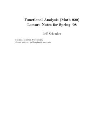
LECTURE 2Geometric Hahn-Banach TheoremsReading: §3.2, §3.3 of Lax.We may use Hahn-Banach to understand something of the geometry of linear spaces. Wewant to understand if the following picture holds in infinite dimension:Figure 2.1. Separating a point from a convex set by a line hyperplaneDefinition 2.1. A set S X is convex if for all x, y S and t [0, 1] we havetx (1 t)y S.Definition 2.2. A point x S X is an interior point of S if for all y X ε 0 s.t. t ε x ty S.Remark. We can a define a topology using this notion, letting U X be open all x U are interior. From the standpoint of abstract linear algebra this seems to bea “natural” topology on X. In practice, however, it has way too many open sets and wework with weaker topologies that are relevant to the analysis under considerations. Much offunctional analysis centers around the interplay of different topologies.We are aiming at the following2-1
2-22. GEOMETRIC HAHN-BANACH THEOREMSTheorem 2.1. Let K be a non-empty convex subset of X, a linear space over R, andsuppose K has at least one interior point. If y 6 K then a linear functional : X R s.t. (x) (y) for all x K,(2.1)with strict inequality for all interior points x of K.This is the “hyperplane separation theorem,” essentially validates the picture drawnabove. A set of the form { (x) c} with a linear functional is a “hyperplane” and the sets{ (x) c} are “half spaces.”To accomplish the proof we will use Hahn-Banach. We need a dominating function p.Definition 2.3. Let K X be convex and suppose 0 is an interior point. The gaugeof K (with respect to the origin) is the function pK : X R defined asxpK (x) inf{a : a 0 and K}.a(Note that pK (x) for all x since 0 is interior.)Lemma 2.2. pK is positive homogeneous and sub-additive.Proof. Positive homogeneity is clear (even if K is not convex). To prove sub-additivitywe use convexity. Consider pK (x y). Let a, b be such that x/a, y/b K. Thenxyt (1 t) K t [0, 1],absox ya xb y K.a ba ba a bbThus pK (x y) a b, and optimizing over a, b we obtain the result. Proof of hyperplane separation thm. Suffices to assume 0 K is interior andc 1. Let pK be the gauge of K. Note that pK (x) 1 for x K and that pK (x) 1 if x isinterior, as then (1 t)x K for small t 0. Conversely if pK (x) 1 then x is an interiorpoint (why?), sopK (x) 1 x K.Now define (y) 1, so (ay) a for a R. Since y 6 K it is not an interior point andso pK (y) 1. Thus pK (ay) a for a 0 and also, trivially, for a 0 (since pK 0). ThuspK (ay) (ay)for all a R. By Hahn-Banach, with Y the one dimensional space {ay}, may be extendedto all of x so that pK (x) (x) which implies (2.1). An extension of this is the followingTheorem 2.3. Let H, M be disjoint convex subsets of X, at least one of which has aninterior point. Then H and M can be separate by a hyperplane (x) c: there is a linearfunctional and c R such that (u) c (v) u H, v M.
2. GEOMETRIC HAHN-BANACH THEOREMS2-3Proof. The proof rests on a trick of applying the hyperplane separation theorem withthe setK H M {u v : u H and v M }and the point y 0. Note that 0 6 K since H M . Since K has an interior point(why?), we see that there is a linear functional such that (x) 0 for all x K. But then (u) (v) for all u H, v M . In many applications, one wants to consider a vector space X over C. Of course, then Xis also a vector space over R so the real Hahn-Banach theorem applies. Using this one canshow the followingTheorem 2.4 (Complex Hahn-Banach, Bohenblust and Sobczyk (1938) and Soukhomlinoff (1938)). Let X be a linear space over C and p : X [0, ) such that(1) p(ax) a p(x) a C, x X.(2) p(x y) p(x) p(y) (sub-additivity).Let Y be a C linear subspace of X and : Y C a linear functional such that (y) p(y)(2.2)for all y Y . Then can be extended to all of X so that (2.2) holds for all y X.Remark. A function p that satisfies (1) and (2) is called a semi-norm. It is a norm ifp(x) 0 x 0.Proof. Let 1 (y) Re (y), the real part of . Then 1 is a real linear functional and 1 (iy) Re i (y) Im (y), the imaginary part of . Thus (y) 1 (y) i 1 (iy).(2.3)Clearly 1 (y) p(y) so by the real Hahn-Banach theorem we can extend 1 to all ofX so that 1 (y) p(y) for all y X. Since 1 (y) 1 ( y) p( y) p(y), we have 1 (y) p(y) for all y X. Now define the extension of via (2.3). Given y X letθ arg ln (y). Thus (y) eiθ 1 (e iθ y) (why?). So, (y) 1 (e iθ y) p(y). Lax gives another beautiful extension of Hahn-Banach, due to Agnew and Morse, whichinvolves a family of commuting linear maps. We will cover a simplified version of this nexttime.
LECTURE 3Applications of Hahn-BanachReading: §4.1, §4.2 of Lax.To get an idea what one can do with the Hahn-Banach theorem let’s consider a concreteapplication on the linear space X B(S) of all real valued bounded functions on a set S.B(S) has a natural partial order, namely x y if x(s) y(s) for all s S. If 0 x then xis nonnegative. On B(S) a positive linear functional satisfies (y) 0 for all y 0.Theorem 3.1. Let Y be a linear subspace of B(S) that contains y0 1, so y0 (s) 1for all s S. If is a positive linear functional on Y then can be extended to all of B asa positive linear functional.This theorem can be formulated in an abstract context as follows. The nonnegativefunctions form a cone, whereDefinition 3.1. A subset P X of a linear space over R is a cone if tx sy Pwhenever x, y P and t, s 0. A linear functional on X is P -nonnegative if (x) 0 forall x P .Theorem 3.2. Let P X be a cone with an interior point x0 . If Y is a subspacecontaining x0 on which is defined a P Y -positive linear functional , then has an extensionto X which is P -positive.Proof. Define a dominating function p as followsp(x) inf{ (y) : y x P, y Y }.Note that y0 tx P for some t 0 (since y0 is interior to P ), so 1t y0 x P . Thisshows that p(x) is well defined. It is clear that p is positive homegeneous. To see that it issub-additive, let x1 , x2 X and let y1 , y2 be so that yj xj P . Then y1 y2 (x1 x2 ) P ,sop(x1 x2 ) (y1 ) (y2 ).Minimizing over y1,2 gives sub-additivity.Since (x) (x y) (y) (y) if x Y and y x P we conclude that (x) p(x)for all x Y . By Hahn-Banach we may extend to all of X so that (x) p(x) for all x.Now let x P . Then p( x) 0 (why?), so (x) ( x) 0 which shows that isP -positive. The theorem on B(S) follows from the Theorem 3.2 once we observe that the conditiony0 1 implies that y0 is an interior point of the cone of positive functions. The linearfunctional that one constructs in this way is monotone:x y (x) (y),which is in fact equivalent to positivity. This can allow us to do a little bit of analysis, eventhough we haven’t introduced notions of topology or convergence.3-1
3-23. APPLICATIONS OF HAHN-BANACHTo see how this could work, let’s apply the result to the Riemann integral on C[0, 1].conclude the existence of a positive linear functional : B[0, 1] R that gives (f ) RWe1f (x)dx. This gives an “integral” of arbitrary bounded functions, without a measurability0condition. Since the integral is a linear functional, it is finitely additive. Of course it isnot countably additive since we know from real analysis that such a thing doesn’t exist.Furthermore, the integral is not uniquely defined.Nonetheless, the extension is also not arbitrary, and the constraint of positivity actuallypins down (f ) for many functions. For example, consider χ(a,b) (the characteristic functionof an open interval). By positivity we know thatZ 1Z 1g(x)dx.f (x)dx (χ(a,b) ) f χ(a,b) g, f, g C[0, 1] 00Taking the sup over f and inf over g, using properties only of the Riemann integral, we seethat (χ(a,b) ) b a (hardly a surprising result). Likewise, we can see that (χU ) U forany open set, and by finite additivity (χF ) 1 (F c ) 1 F c F for any closed set( · is Lebesgue measure). Finally if S [0, 1] andsup { (F ) : F closed and F S} inf { (U ) : U open and U S}then (χS ) must be equal to these two numbers. We see that (χS ) S for any Lebesguemeasurable set. We have just painlessly constructed Lebesgue measure from the Riemannintegral without using any measure theory!The rigidity of the extension is a bit surprising if we compare with what happens infinite dimensions. For instance, consider the linear functional (x, 0) x defined on Y {(x, 0)} R2 . Let P be the cone {(x, y) : y αx}. So is P Y -positive. To extend to all of R2 we need to define (0, 1). To keep the extension positive we need only requirey (0, 1) 1 0if y α. Thus we must have (0, 1) 1/α, and any choice in this interval will work.Only when α and the cone degenerates to a half space does the condition pin (0, 1)down. So some interesting things happen in dimensions.A second example application assigning a limiting value to sequencesa (a1 , a2 , . . .).Let B denote the space of all bounded R-valued sequences and let L denote the subspace ofsequences with a limit. We quickly conclude that there is an positive linear extension of thepositive linear functional lim to all of B. We would like to conclude a little more, however.After all, for convergent sequences,lim an k lim anfor any k.To formalize this property we define a linear map on B byT (a1 , a2 , . . .) (a2 , a3 , . . .).(T is the “backwards shift” operator or “left translation.”) Here,Definition 3.2. Let X1 , X2 be linear spaces over a field F . A linear map T : X1 X2is a function such thatT (x ay) T (x) aT (y) x, y X1 and a F.
3. APPLICATIONS OF HAHN-BANACH3-3Thus lim T a lim a for a L. We would like the extension to have this property. Canthis be done?The answer is given by the following a simplified version of the Theorem of Agnew andMorse given in Chapter 3 of Lax:Theorem 3.3. Let X be a linear space over R and let T : X X be a linear map. Letp : X R be a positive homogeneous, sub-additive function invariant under T :p(T x) p(x) x X.Let be a linear functional defined on a subspace Y X invariant under T ,Ty Y y Y.If is invariant under T — (T y) (y) — and dominated by p then may be extended toall of X so that the extension is also invariant under T and dominated by p.Remark. Applying this to the space B of bounded sequences and lettingp(a) lim sup a,we find that there is an extension of the linear functional lim from L to all of B such thatfor all a (a1 , a2 , . . .)(1) limn an k limn an for all k.(2) lim inf a lim a lim sup a . (The first inequality follows from the second appliedto a.)Proof. Let us defineq(x) inf p(Ax),where the infimum is over all convex combinations of powers of T ,nXA aj T j(3.1)j 0wherePT 0 1, the identity operator on X, 1x x, and aj is any finite, non-negative sequencewith j aj 1. Clearly q(x) is positive homogeneous and q(x) p(x). Also, since and Yare invariant under any A of the form (3.1) we have (y) q(y) y Y.To apply Hahn-Banach with q as the dominating function we need to show it is subadditivie. To this end, let x, y X and let A, B be of the form (3.1) so thatp(Ax) q(x) and p(By) q(y) .Then A B B A is of the form (3.1) andq(x y) p(AB(x y)) p(BAx) p(ABy) p(Ax) p(By) q(x) q(y) 2 .Thus q is sub-additive.So now we know that an extension exists to all of X with (x) q(x) for all x. However,!n1X j11q(x T x) pT (1 T )x p(x T n 1 x) (p(x) p( x)) 0.n j 0nnSo q(x T x) 0 for all x and thus (x) (T x) 0 for all x.
Part 2Banach Spaces
LECTURE 4Normed and Banach SpacesReading: §5.1 of Lax.The Hahn-Banach theorem made use of a dominating function p(x). When this functionis non-negative, it can be understood roughly as a kind of “distance” from a point x to theorigin. For that to work, we should have p(x) 0 whenever x 6 0. Such a function is calleda norm:Definition 4.1. Let X be a linear space over F R or C. A norm on X is a functionk·k : X [0, ) such that(1) kxk 0 x 0.(2) kx yk kxk kyk (subadditivity)(3) kaxk a kxk for all a F and x X (homogeneity).A normed space is a linear space X with a norm k·k.The norm on a normed space gives a metric topology if we define the distance betweentwo points viad(x, y) kx yk .Condition 1 guarantees that two distinct points are a finite distance apart. Sub-additivitygives the triangle inequality. The metric is(1) translation invariant: d(x z, y z) d(x, y)and(2) homogeneous d(ax, ay) a d(x, y).Thus any normed space is a metric space and we have the following notions:(1)(2)(3)(4)aaaasequence xn converges to x, xn x, if d(xn , x) kxn xk 0.set U X is open if for every x U there is a ball {y : ky xk } U .set K X is closed if X \ K is open.set K X is compact if every open cover of K has a finite sub-cover.The norm defines the topology but not the other way around. Indeed two norms k·k1and k·k2 on X are equivalent if there is c 0 such thatc kxk1 kxk2 c 1 kxk2 x X.Equivalent norms define the same topology. (Why?)Recall from real analysis that a metric space X is complete if every Cauchy sequence xnconverges in X. In a normed space, a Cauchy sequence xn is one such that 0 N N such that n, m N kxn xm k .A complete normed space is called a Banach space.4-1
4-24. NORMED AND BANACH SPACESNot every normed space is complete. For example C[0, 1] with the normZ 1kf k1 f (x) dx0fails to be complete. (It is, however, a complete space in the uniform norm, kf ku supx [0,1] f (x) .) However, every normed space X has a completion, defined abstractly asa set of equivalence classes of Cauchy sequences in X. This space, denoted X is a Banachspace.Examples of Normed and Banach spaces(1) For each p [1, ) let p {p summable sequences} {(a1 , a2 , . . .) X aj p }.j 1Define a norm on p via"kakp X# p1 aj p.j 1Then p is a Banach space.(2) Let {bounded sequences} B(N),with normkak sup aj .(?)jThen is a Banach space.(3) Letc0 {sequences converging to 0} {(a1 , a2 , . . .) lim aj 0},j with norm (?). Then c0 is a Banach space.(4) LetF {sequences with finitely many non-zero terms} {(a1 , a2 , . . .) N N such that n N an 0}.Then for any p 1, Fp (F, k·kp ) is a normed space which is not complete. Thecompletion of Fp is isomorphic to p .(5) Let D Rd be a domain and let p [1, ).(a) Let X Cc (D) be the space of continuous functions with compact support inD, with the norm Z p1pkf kp f (x) dx .D
EXAMPLES OF NORMED AND BANACH SPACES4-3Then X is a normed space, which is not complete. Its completion is denotedLp (D) and may be identified with the set of equivalence classes of measurablefunctions f : D C such thatZ f (x) p dx (Lebesgue measure),Dwith two functions f, g called equivalent if f (x) g(x) for almost every x.(b) Let X denote the set of C 1 functions on D such thatZZp f (x) dx and j f (x) p dx , j 1, . . . , n.DDPut the following norm on X,"Z# p1n ZXkf k1,p f (x) p dx j f (x) p dx. .Dj 1DThen X is a normed space which is not complete. Its completion is denotedW 1,p (D) and is called a Sobolev space and may be identified with the subspace of Lp (D) consisting of (equivalence classes) of functions all of whose firstderivatives are in Lp (D) in the sense of distributions. (We’ll come back to this.)Note that a 1 is summable,Xaj kak1 .jTheorem 4.1 (Hölder’s Inqequality). Let 1 p and let q be such that1 1 1.p qIf a p and b q thenab (a1 b1 , a2 b2 , . . .) 1and Xaj bj kakp kbkq .j 1Proof. First note that for two non-negative numbers a, b it holds that11ab ap bq .pqFor p q 2 this is the familiar “arithmetic-geometric mean” inequality which follows since(a b)2 0. For general a, b this may be seen as follows. The function x 7 exp(x) is convex:exp(tx (1 t)y) t exp(x) (1 t) exp(y). (Recall from calculus that a C 2 function f isconvex if f 00 0.) Thus,111111ab exp( ln ap ln bq ) exp(ln ap ) exp(ln bq ) ap bq .pqpqpqApplying this bound co-ordinate wise and summing up we find that11kabk1 kakpp kbkqq .pq
4-44. NORMED AND BANACH SPACESThe result follows from this bound by “homogenization:” we havekakp , kbkq kabk 1,soabkakp kbkq 11from which the desired estimate follows by homogeneity of the norm. Similarly, we haveTheorem 4.2 (Hölder’s Inequality). Let 1 p and let q be the conjugate exponent.If f Lp (D) and g Lq (D) then f g L1 (D) andZ f (x)g(x) dx kf kp kgkq .D
LECTURE 5Noncompactness of the Ball and Uniform ConvexityReading: §5.1 and §5.2 of Lax.First a few more definitions:Definition 5.1. A normed space X over F R or C is called separable if it has acountable, dense subset.Most spaces we consider are separable, with a few notable exceptions.(1) The space M of all signed (or complex) measures µ on [0, 1], say, with normZ 1kµk µ (dx).0Here µ denotes the total variation of µ, µ (A) supnX µ(Aj ) .Partitions A1 , . . . , An of A j 1This space is a Banach space. Since the point mass(1 x Aδx (A) 0 x 6 Ais an element of A and kδx δy k 2 if x 6 y, we have an uncountable family ofelements of M all at a fixed distance of one another. Thus there can be no countabledense subset. (Why?)(2) is also not separable. To see this, note that to each subset of A N we mayassociate the sequence χA , andkχA χB k 1if A 6 B.(3) p is separable for 1 p .(4) Lp (D) is separable for 1 p .(5) L (D) is not separable.Noncompactness of the Unit BallTheorem 5.1 (F. Riesz). Let X be a normed linear space. Then the closed unit ballB1 (0) {x : kXk 1} is compact if and only if X is finite dimensional.Proof. The fact that the unit ball is compact if X is finite dimensional is the HeineBorel Theorem from Real Analysis.To see the converse, we use the following5-1
5-25. NONCOMPACTNESS OF THE BALL AND UNIFORM CONVEXITYLemma 5.2. Let Y be a closed proper subspace of a normed space X. Then there is aunit vector z X, kzk 1, such that1 y Y.2Proof of Lemma. Since Y is proper, x X \ Y . Thenkz yk inf kx yk d 0.y Y(This is a property of closed sets in a metric space.) We do not know the existence of aminimizing y, but we can certainly find y0 such that0 kx y0 k 2d.Let z x y0.kx y0 kThenkz yk d1kx y0 kx y0 k yk .kx y0 k2d2 Returning to the proof of the Theorem, we will use the fact that every sequence in acompact metric space has a convergent subsequence. Thus it suffices to show that if X isinfinite dimensional then there is a sequence in B1 (0) with no convergent subsequence.Let y1 be any unit vector and construct a sequence of unit vectors, by induction, so that1kyk yk y span{y1 , . . . , yk 1 }.2(Note that span{y1 , . . . , yk 1 } is finite dimensional, hence complete, and thus a closed subspace of X.) Since X is finite dimensional the process never stops. No subsequence of yjcan be Cauchy, much less convergent. Uniform convexityThe following theorem may be easily shown using compactness:Theorem 5.3. Let X be a finite dimensional linear normed space. Let K be a closedconvex subset of X and z any point of X. Then there is a unique point of K closer to z thanany other point of K. That is there is a unique solution y0 K to the minimization problemky0 zk inf ky zk .y K(?)Try to prove this theorem. (The existence of a minimizer follows from compactness; theuniqueness follows from convexity.)The conclusion of theorem does not hold in a general infinite dimensional space. Nonetheless there is a property which allows for the conclusion, even though compactness fails!Definition 5.2. A normed linear space X is uniformly convex if there is a function : (0, ) (0, ), such that(1) is increasing.(2) limr 0 (r) 0.(3) 12 (x y) 1 (kx yk) for all x, y B1 (0), the unit ball of X.
UNIFORM CONVEXITY5-3Theorem 5.4 (Clarkson 1936). Let X be a uniformly convex Banach space, K a closedconvex subset of X, and z any point of X. Then the minimization problem (?) has a uniquesolution y0 K.Proof. If z K then y0 z is the solution, and is clearly unique.When z 6 K, we may assume z 0 (translating z and K if necessary). Lets inf kyk .y KSo s 0. Now let yn K be a minimizing sequence, sokyn k s.Now let xn yn / kyn k, and consider111(xn xm ) yn ym 22
functional analysis centers around the interplay of di erent topologies. We are aiming at the following 2-1. 2-2 2. GEOMETRIC HAHN-BANACH THEOREMS Theorem 2.1. Let K be a non-empty convex subset of X, a linear space over R, and suppose Khas at least one int