Transcription
Algebra II Chapterof theMathematics Frameworkfor California Public Schools:Kindergarten Through Grade TwelveAdopted by the California State Board of Education, November 2013Published by the California Department of EducationSacramento, 2015
Algebra IITAlgebra IIGeometryAlgebra Ihe Algebra II course extends students’ understandingof functions and real numbers and increases the toolsstudents have for modeling the real world. Students inAlgebra II extend their notion of number to include complexnumbers and see how the introduction of this set of numbersyields the solutions of polynomial equations and the Fundamental Theorem of Algebra. Students deepen their understanding of the concept of function and apply equation-solvingand function concepts to many different types of functions. Thesystem of polynomial functions, analogous to integers, isextended to the field of rational functions, which is analogousto rational numbers. Students explore the relationship betweenexponential functions and their inverses, the logarithmicfunctions. Trigonometric functions are extended to all realnumbers, and their graphs and properties are studied. Finally,students’ knowledge of statistics is extended to include understanding the normal distribution, and students are challengedto make inferences based on sampling, experiments, andobservational studies.For the Traditional Pathway, the standards in the Algebra IIcourse come from the following conceptual categories: Modeling, Functions, Number and Quantity, Algebra, and Statisticsand Probability. The course content is explained below according to these conceptual categories, but teachers and administrators alike should note that the standards are not listedhere in the order in which they should be taught. Moreover,the standards are not simply topics to be checked off from alist during isolated units of instruction; rather, they representcontent that should be present throughout the school year inrich instructional experiences.California Mathematics FrameworkAlgebra II473
What Students Learn in Algebra IIBuilding on their work with linear, quadratic, and exponential functions, students in Algebra II extendtheir repertoire of functions to include polynomial, rational, and radical functions.1 Students work closelywith the expressions that define the functions and continue to expand and hone their abilities to modelsituations and to solve equations, including solving quadratic equations over the set of complex numbersand solving exponential equations using the properties of logarithms. Based on their previous workwith functions, and on their work with trigonometric ratios and circles in Geometry, students now usethe coordinate plane to extend trigonometry to model periodic phenomena. They explore the effects oftransformations on graphs of diverse functions, including functions arising in applications, in order toabstract the general principle that transformations on a graph always have the same effect regardless ofthe type of underlying function. They identify appropriate types of functions to model a situation, adjustparameters to improve the model, and compare models by analyzing appropriateness of fit and makingjudgments about the domain over which a model is a good fit. Students see how the visual displays andsummary statistics learned in earlier grade levels relate to different types of data and to probabilitydistributions. They identify different ways of collecting data—including sample surveys, experiments,and simulations—and the role of randomness and careful design in the conclusions that can be drawn.Examples of Key Advances from Previous Grade Levels or Courses In Algebra I, students added, subtracted, and multiplied polynomials. Students in Algebra II dividepolynomials that result in remainders, leading to the factor and remainder theorems. This is theunderpinning for much of advanced algebra, including the algebra of rational expressions. Themes from middle-school algebra continue and deepen during high school. As early as grade six,students began thinking about solving equations as a process of reasoning (6.EE.5). This perspectivecontinues throughout Algebra I and Algebra II (A-REI). “Reasoned solving” plays a role in Algebra IIbecause the equations students encounter may have extraneous solutions (A-REI.2). In Algebra I, students worked with quadratic equations with no real roots. In Algebra II, they extendtheir knowledge of the number system to include complex numbers, and one effect is that theynow have a complete theory of quadratic equations: Every quadratic equation with complexcoefficients has (counting multiplicity) two roots in the complex numbers. In grade eight, students learned the Pythagorean Theorem and used it to determine distances in acoordinate system (8.G.6–8). In the Geometry course, students proved theorems using coordinates(G-GPE.4–7). In Algebra II, students build on their understanding of distance in coordinate systemsand draw on their growing command of algebra to connect equations and graphs of conic sections(for example, refer to standard G-GPE.1). In Geometry, students began trigonometry through a study of right triangles. In Algebra II, theyextend the three basic functions to the entire unit circle. As students acquire mathematical tools from their study of algebra and functions, they apply thesetools in statistical contexts (for example, refer to standard S-ID.6). In a modeling context, studentsmight informally fit an exponential function to a set of data, graphing the data and the model functionon the same coordinate axes (Partnership for Assessment of Readiness for College and Careers 2012).1. In this course, rational functions are limited to those with numerators having a degree not more than 1 and denominatorshaving a degree not more than 2; radical functions are limited to square roots or cube roots of at most quadratic polynomials (National Governors Association Center for Best Practices, Council of Chief State School Officers [NGA/CCSSO] 2010a).474Algebra IICalifornia Mathematics Framework
Connecting Mathematical Practices and ContentThe Standards for Mathematical Practice (MP) apply throughout each course and, together with theStandards for Mathematical Content, prescribe that students experience mathematics as a coherent,relevant, and meaningful subject. The Standards for Mathematical Practice represent a picture of whatit looks like for students to do mathematics and, to the extent possible, content instruction shouldinclude attention to appropriate practice standards. There are ample opportunities for students toengage in each mathematical practice in Algebra II; table A2-1 offers some general examples.Table A2-1. Standards for Mathematical Practice—Explanation and Examples for Algebra IIStandards for MathematicalPracticeExplanation and ExamplesMP.1Students apply their understanding of various functions to real-worldproblems. They approach complex mathematics problems and breakMake sense of problems andthem down into smaller problems, synthesizing the results whenpersevere in solving them.presenting solutions.MP.2Students deepen their understanding of variables—for example, byReason abstractly and quantitatively. understanding that changing the values of the parameters in thehas consequences for the graph of theexpressionfunction. They interpret these parameters in a real-world context.MP.3Students continue to reason through the solution of an equation andjustifytheir reasoning to their peers. Students defend their choice ofConstruct viable arguments anda function when modeling a real-world situation.critique the reasoning of others.Students build proofs by inductionand proofs by contradiction. CA 3.1(for higher mathematics only).MP.4Model with mathematics.MP.5Use appropriate tools strategically.MP.6Attend to precision.MP.7Look for and make use of structure.Students apply their new mathematical understanding to real-worldproblems, making use of their expanding repertoire of functions inmodeling. Students also discover mathematics through experimentation and by examining patterns in data from real-world contexts.Students continue to use graphing technology to deepen their understanding of the behavior of polynomial, rational, square root, andtrigonometric functions.Students make note of the precise definition of complex number,understanding that real numbers are a subset of complex numbers.They pay attention to units in real-world problems and use unitanalysis as a method for verifying their answers.Students see the operations of complex numbers as extensions of theoperations for real numbers. They understand the periodicity of sineand cosine and use these functions to model periodic phenomena.(Table continues on next page)California Mathematics FrameworkAlgebra II475
Table A2-1 (continued)MP.8Students observe patterns in geometric sums—for example, that theLook for and express regularity inrepeated reasoning.first several sums of the formcan be written as follows:Students use this observation to make a conjecture about any such sum.Standard MP.4 holds a special place throughout the higher mathematics curriculum, as Modeling isconsidered its own conceptual category. Although the Modeling category does not include specificstandards, the idea of using mathematics to model the world pervades all higher mathematics coursesand should hold a significant place in instruction. Some standards are marked with a star ( ) symbolto indicate that they are modeling standards—that is, they may be applied to real-world modelingsituations more so than other standards. In the description of the Algebra II content standards thatfollow, Modeling is covered first to emphasize its importance in the higher mathematics curriculum.Examples of places where specific Mathematical Practice standards can be implemented in the AlgebraII standards are noted in parentheses, with the standard(s) also listed.Algebra II Content Standards, by Conceptual CategoryThe Algebra II course is organized by conceptual category, domains, clusters, and then standards. Theoverall purpose and progression of the standards included in Algebra II are described below, according to each conceptual category. Standards that are considered new for secondary-grades teachers arediscussed more thoroughly than other standards.Conceptual Category: ModelingThroughout the California Common Core State Standards for Mathematics (CA CCSSM), specific standardsfor higher mathematics are marked with a symbol to indicate they are modeling standards. Modelingat the higher mathematics level goes beyond the simple application of previously constructed mathematics and includes real-world problems. True modeling begins with students asking a question aboutthe world around them, and the mathematics is then constructed in the process of attempting to answerthe question. When students are presented with a real-world situation and challenged to ask a question,all sorts of new issues arise: Which of the quantities present in this situation are known and unknown?Can a table of data be made? Is there a functional relationship in this situation? Students need to decideon a solution path, which may need to be revised. They make use of tools such as calculators, dynamicgeometry software, or spreadsheets. They try to use previously derived models (e.g., linear functions),but may find that a new equation or function will apply. In addition, students may see when trying toanswer their question that solving an equation arises as a necessity and that the equation often involvesthe specific instance of knowing the output value of a function at an unknown input value.476Algebra IICalifornia Mathematics Framework
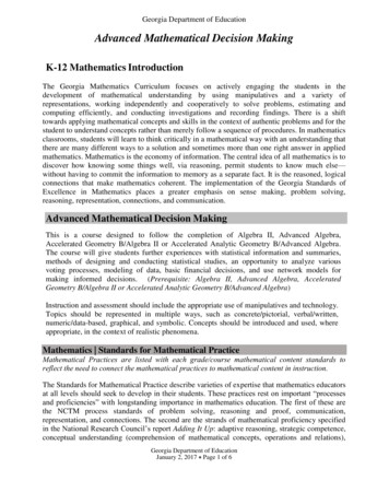
Modeling problems have an element of being genuine problems, in the sense that students care aboutanswering the question under consideration. In modeling, mathematics is used as a tool to answerquestions that students really want answered. Students examine a problem and formulate a mathematical model (an equation, table, graph, or the like), compute an answer or rewrite their expression toreveal new information, interpret and validate the results, and report out; see figure A2-1. This is a newapproach for many teachers and may be challenging to implement, but the effort should show studentsthat mathematics is relevant to their lives. From a pedagogical perspective, modeling gives a concretebasis from which to abstract the mathematics and often serves to motivate students to becomeindependent learners.Figure A2-1. The Modeling tThe examples in this chapter are framed as much as possible to illustrate the concept of mathematicalmodeling. The important ideas surrounding polynomial and rational functions, graphing, trigonometricfunctions and their inverses, and applications of statistics are explored through this lens. Readers areencouraged to consult appendix B (Mathematical Modeling) for further discussion of the modeling cycleand how it is integrated into the higher mathematics curriculum.Conceptual Category: FunctionsWork on functions began in Algebra I. In Algebra II, students encounter more sophisticated functions,such as polynomial functions of degree greater than 2, exponential functions having all real numbersas the domain, logarithmic functions, and extended trigonometric functions and their inverses. Severalstandards of the Functions category are repeated here, illustrating that the standards attempt to reachdepth of understanding of the concept of a function. As stated in the University of Arizona (UA) Progressions Documents for the Common Core Math Standards, “students should develop ways of thinking thatare general and allow them to approach any function, work with it, and understand how it behaves,rather than see each function as a completely different animal in the bestiary” (UA Progressions Documents 2013c, 7). For instance, students in Algebra II see quadratic, polynomial, and rational functionsas belonging to the same system.California Mathematics FrameworkAlgebra II477
Interpreting FunctionsF-IFInterpret functions that arise in applications in terms of the context. [Emphasize selection of appropriate models.]4. For a function that models a relationship between two quantities, interpret key features of graphs andtables in terms of the quantities, and sketch graphs showing key features given a verbal description of therelationship. Key features include: intercepts; intervals where the function is increasing, decreasing, positive,or negative; relative maximums and minimums; symmetries; end behavior; and periodicity. 5. Relate the domain of a function to its graph and, where applicable, to the quantitative relationship itdescribes. 6. Calculate and interpret the average rate of change of a function (presented symbolically or as a table)over a specified interval. Estimate the rate of change from a graph. Analyze functions using different representations. [Focus on using key features to guide selection ofappropriate type of model function.]7. Graph functions expressed symbolically and show key features of the graph, by hand in simple cases andusing technology for more complicated cases. b. Graph square root, cube root, and piecewise-defined functions, including step functions and absolutevalue functions. c. Graph polynomial functions, identifying zeros when suitable factorizations are available, and showingend behavior. e. Graph exponential and logarithmic functions, showing intercepts and end behavior, and trigonometric functions, showing period, midline, and amplitude. 8. Write a function defined by an expression in different but equivalent forms to reveal and explain differentproperties of the function.9. Compare properties of two functions each represented in a different way (algebraically, graphically,numerically in tables, or by verbal descriptions).In this domain, students work with functions that model data and choose an appropriate model function by considering the context that produced the data. Students’ ability to recognize rates of change,growth and decay, end behavior, roots, and other characteristics of functions is becoming more sophisticated; they use this expanding repertoire of families of functions to inform their choices for models.This group of standards focuses on applications and how key features relate to characteristics of asituation, making selection of a particular type of function model appropriate (F-IF.4–9). The followingexample illustrates some of these standards.478Algebra IICalifornia Mathematics Framework
Example: The Juice CanF-IF.4–5; F-IF.7–9Students are asked to find the minimal surface area of a cylindrical can of a fixed volume. The surface areais represented in units of square centimeters (cm2 ), the radius in units of centimeters (cm), and the volumeis fixed at 355 milliliters (ml), or 355 cm3. Students can find the surface area of this can as a function of theradius:(See The Juice-Can Equation example that appears in the Algebra conceptual category of this chapter.)This representation allows students to examine several things. First, a table of values will provide a hint aboutwhat the minimal surface area is. The table below lists several values for based on 0284.9299.0319.1344.4374.6409.1447.9490.7Continued on next pageCalifornia Mathematics FrameworkAlgebra II479
Example: The Juice Can (continued)The data suggest that the minimal surface area occurs when the radius of the base of the juice can is between3.5 and 4.5 centimeters. Successive approximation using values of between these values will yield a better estimate. But how can students be sure that the minimum is truly located here? A graph ofprovides a clue:200010000510Furthermore, students can deduce that as gets smaller, the termtermgets larger and larger, while thegets smaller and smaller, and that the reverse is true as grows larger, so that there is truly a mini-mum somewhere in the interval.Graphs help students reason about rates of change of functions (F-IF.6). In grade eight, studentslearned that the rate of change of a linear function is equal to the slope of the graph of that function.And because the slope of a line is constant, the phrase “rate of change” is clear for linear functions.For non-linear functions, however, rates of change are not constant, and thus average rates of changeover an interval are used. For example, for the function defined for all real numbers by,the average rate of change fromtois.This is the slope of the line containing the pointsandon the graph of . If is interpretedas returning the area of a square of side length , then this calculation means that over this interval thearea changes, on average, by 7 square units for each unit increase in the side length of the square (UAProgressions Documents 2013c, 9). Students could investigate similar rates of change over intervals forthe Juice Can problem shown previously.480Algebra IICalifornia Mathematics Framework
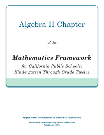
Building FunctionsF-BFBuild a function that models a relationship between two quantities. [Include all types of functionsstudied.]1. Write a function that describes a relationship between two quantities. b. Combine standard function types using arithmetic operations. For example, build a function thatmodels the temperature of a cooling body by adding a constant function to a decaying exponential, andrelate these functions to the model. Build new functions from existing functions. [Include simple radical, rational, and exponentialfunctions; emphasize common effect of each transformation across function types.]3. Identify the effect on the graph of replacingby,,, andfor specificvalues of (both positive and negative); find the value of given the graphs. Experiment with cases andillustrate an explanation of the effects on the graph using technology. Include recognizing even and oddfunctions from their graphs and algebraic expressions for them.4. Find inverse functions.for a simple functiona. Solve an equation of the formexpression for the inverse. For example,orthat has an inverse and write anfor.Students in Algebra II develop models for more complex situations than in previous courses, due tothe expansion of the types of functions available to them (F-BF.1). Modeling contexts provide a naturalplace for students to start building functions with simpler functions as components. Situations in whichcooling or heating are considered involve functions that approach a limiting value according to a decaying exponential function. Thus, if the ambient room temperature is 70 degrees Fahrenheit and a cup oftea is made with boiling water at a temperature of 212 degrees Fahrenheit, a student can express thefunction describing the temperature as a function of time by using the constant functiontorepresent the ambient room temperature and the exponentially decaying functiontorepresent the decaying difference between the temperature of the tea and the temperature of theroom, which leads to a function of this form:Students might determine the constant experimentally (MP.4, MP.5).Example: Population GrowthF-BF.1The approximate population of the United States, measured each decade starting in 1790 through 1940, canbe modeled with the following function:In this function, represents the number of decades after 1790. Such models are important for planninginfrastructure and the expansion of urban areas, and historically accurate long-term models have beendifficult to derive.Continued on next pageCalifornia Mathematics FrameworkAlgebra II481
Example: Population Growth (continued)y14y Q( t )13U.S. Population in Tens of Millions121110987654321123456789 10 11 12 13 14 15tNumber of Decades after 1790Questions:a. According to this model, what was the population of the United States in the year 1790?b. According to this model, when did the U.S. population first reach 100,000,000? Explain your answer.c. According to this model, what should the U.S. population be in the year 2010? Find the actual U.S.population in 2010 and compare with your result.d. For larger values of , such asfindings., what does this model predict for the U.S. population? Explain yourSolutions:a. The population in 1790 is given by, which is easily found to be 3,900,000 becauseb. This question asks students to find such that. Dividing the numerator and denom-inator on the left by 100,000,000 and dividing both sides of the equation by 100,000,000 simplifies thisequation to.Algebraic manipulation and solving for result in. This means that after 1790, itwould take approximately 126.4 years for the population to reach 100 million.c. Twenty-two (22) decades after 1790, the population would be approximately 190,000,000, which is farless (by about 119,000,000) than the estimated U.S. population of 309,000,000 in 2010.d. The structure of the expression reveals that for very large values of , the denominator is dominated by. Thus, for very large values of ,.Therefore, the model predicts a population that stabilizes at 200,000,000 as increases.Adapted from Illustrative Mathematics 2013m.482Algebra IICalifornia Mathematics Framework
Students can make good use of graphing software to investigate the effects of replacing a functionby,,, andfor different types of functions (MP.5). For example,starting with the simple quadratic function, students see the relationship between thesetransformed functions and the vertex form of a general quadratic,. They understand the notion of a family of functions and characterize such function families based on theirproperties. These ideas are explored further with trigonometric functions (F-TF.5).With standard F-BF.4a, students learn that some functions have the property that an input can berecovered from a given output; for example, the equationcan be solved for , given thatlies in the range of . Students understand that this is an attempt to “undo” the function, or to “gobackwards.” Tables and graphs should be used to support student understanding here. This standarddovetails nicely with standard F-LE.4 described below and should be taught in progression with it.Students will work more formally with inverse functions in advanced mathematics courses, and sostandard F-LE.4 should be treated carefully to prepare students for deeper understanding of functionsand their inverses.Linear, Quadratic, and Exponential ModelsF-LEConstruct and compare linear, quadratic, and exponential models and solve problems.4. For exponential models, express as a logarithm the solution towhere , , and are numbersand the base is 2, 10, or ; evaluate the logarithm using technology. [Logarithms as solutions forexponentials]4.1 Prove simple laws of logarithms. CA 4.2 Use the definition of logarithms to translate between logarithms in any base. CA 4.3 Understand and use the properties of logarithms to simplify logarithmic numeric expressions and toidentify their approximate values. CA Students worked with exponential models in Algebra I and continue this work in Algebra II. Since theexponential functionis always increasing or always decreasing for, 1, it can be deducedthat this function has an inverse, called the logarithm to the base , denoted by. Thelogarithm has the property thatif and only if, and this arises in contexts where onewishes to solve an exponential equation. Students find logarithms with base equal to 2, 10, or byhand and using technology (MP.5). Standards F-LE.4.1–4.3 call for students to explore the properties, and students connect these properties to those ofof logarithms, such asexponents (e.g., the previous property comes from the fact that the logarithm represents an exponent). Students solve problems involving exponential functions and logarithms andand thatexpress their answers using logarithm notation (F-LE.4). In general, students understand logarithmsas functions that undo their corresponding exponential functions; instruction should emphasize thisrelationship.California Mathematics FrameworkAlgebra II483
Trigonometric FunctionsF-TFExtend the domain of trigonometric functions using the unit circle.1. Understand radian measure of an angle as the length of the arc on the unit circle subtended by the angle.2. Explain how the unit circle in the coordinate plane enables the extension of trigonometric functions toall real numbers, interpreted as radian measures of angles traversed counterclockwise around the unitcircle.2.1 Graph all 6 basic trigonometric functions. CAModel periodic phenomena with trigonometric functions.5. Choose trigonometric functions to model periodic phenomena with specified amplitude, frequency, andmidline. Prove and apply trigonometric identities.8. Prove the Pythagorean identity sin2 ( ) cos2 ( ) 1 and use it to find sin( ), cos( ), or tan( ) given sin( ),cos( ), or tan( ) and the quadrant of the angle.This set of standards calls for students to expand their understanding of the trigonometric functionsfirst developed in Geometry. At first, the trigonometric functions apply only to angles in right triangles;,, andmake sense only for. By representing right triangles with hypotenuse 1in the first quadrant of the plane, it can be seen that (,) represents a point on the unit circle.This leads to a natural way to extend these functions to any value of that remains consistent with thevalues for acute angles: interpreting as the radian measure of an angle traversed from the point (1,0)counterclockwise around the unit circle,ing to this rotation andis taken to be the -coordinate of the point correspond-to be the -coordinate of this point. This interpretation of sine and cosineimmediately yields the Pythagorean Identity: that. This basic identity yields othersthrough algebraic manipulation and allows values of other trigonometric functions to be found for agiven if one of the values is known (F-TF.1, 2, 8).The graphs of the trigonometric functions should be explored with attention to the connection betweenthe unit-circle representation of the trigonometric functions and their properties—for example, toillustrate the periodicity of the functions, the relationship between the maximums and minimums ofthe sine and cosine graphs, zeros, and so forth. Standard F-TF.5 calls for students to use trigonometricfunctions to model periodic phenomena. This is connected to standard F-BF.3 (families of functions),and students begin to understand the relationship between the parameters appearing in the generalcosine function(and sine function) and the graph and behavior of thefunction (e.g., amplitude, frequency, line of symmetry).484Algebra IICalifornia Mathematics Framework
Example: Modeling Daylight HoursF-TF.5By looking at data for length of days in Columbus, Ohio, students see that the number of daylight hours isapproximately sinusoidal, varying from about 9 hours, 20 minutes on December 21 to about 15 hours on June21. The average of the maximum and minimum gives the value for the midline, and the amplitude is half thedifference of the maximum and minimum. Approximations of these values are set asand.With some support, students determine that for the period to be 365 days (per cycle), or for the frequencyto becycles per day,, and if day 0 corresponds to March 21, no phase shift would be needed, so.Thus,is a function that gives the approximate length of day for , the day of theyear from March 21. Considering questions such as when to plant a garden (i.e., when there are at least 7hours of midday sunlight), students might estimate that a 14-hour day is optimal. Students solveandfind that May 1 and August 10 mark this interval of time. or yfor the frequency to becycles/dayLength of Day (hrs), Columbus, nts can investigate many other trigonometric modeling situations, such as simple predator–pr
In Algebra II, students build on their understanding of distance in coordinate systems and draw on their growing command of algebra to connect equations and graphs of conic sections (for example, refer to standard G-GPE.1). In Geometry, students began trigonometry through a study