Transcription
One Variable Advanced CalculusKenneth KuttlerMarch 9, 2014
2
Contents1 Introduction2 The2.12.22.32.42.52.62.72.82.92.102.112.122.133 Set3.13.23.33.47Real And Complex NumbersThe Number Line And Algebra Of The Real NumbersExercises . . . . . . . . . . . . . . . . . . . . . . . . .Set Notation . . . . . . . . . . . . . . . . . . . . . . .Order . . . . . . . . . . . . . . . . . . . . . . . . . . .Exercises . . . . . . . . . . . . . . . . . . . . . . . . .The Binomial Theorem . . . . . . . . . . . . . . . . .Well Ordering Principle And Archimedean Property .Exercises . . . . . . . . . . . . . . . . . . . . . . . . .Completeness of R . . . . . . . . . . . . . . . . . . . .Existence Of Roots . . . . . . . . . . . . . . . . . . . .Exercises . . . . . . . . . . . . . . . . . . . . . . . . .The Complex Numbers . . . . . . . . . . . . . . . . . .Exercises . . . . . . . . . . . . . . . . . . . . . . . . .TheoryBasic Definitions . . . . . . . . .The Schroder Bernstein TheoremEquivalence Relations . . . . . .Exercises . . . . . . . . . . . . .99131314181920242728293133.35353740414 Functions And Sequences4.1 General Considerations . . . . . . . . . . .4.2 Sequences . . . . . . . . . . . . . . . . . .4.3 Exercises . . . . . . . . . . . . . . . . . .4.4 The Limit Of A Sequence . . . . . . . . .4.5 The Nested Interval Lemma . . . . . . . .4.6 Exercises . . . . . . . . . . . . . . . . . .4.7 Compactness . . . . . . . . . . . . . . . .4.7.1 Sequential Compactness . . . . . .4.7.2 Closed And Open Sets . . . . . . .4.7.3 Compactness And Open Coverings4.8 Exercises . . . . . . . . . . . . . . . . . .4.9 Cauchy Sequences And Completeness . .4.9.1 Decimals . . . . . . . . . . . . . .4.9.2 lim sup and lim inf . . . . . . . . .4.9.3 Shrinking Diameters . . . . . . . .4.10 Exercises . . . . . . . . . . . . . . . . . .4343464749525355555559606264666970.3.
4CONTENTS5 Infinite Series Of Numbers5.1 Basic Considerations . . . . . .5.1.1 Absolute Convergence .5.2 Exercises . . . . . . . . . . . .5.3 More Tests For Convergence . .5.3.1 Convergence Because Of5.3.2 Ratio And Root Tests .5.4 Double Series . . . . . . . . . .5.5 Exercises . . . . . . . . . . . .7575788283838587926 Continuous Functions6.1 Equivalent Formulations Of Continuity . . . . . . . . .6.2 Exercises . . . . . . . . . . . . . . . . . . . . . . . . .6.3 The Extreme Values Theorem . . . . . . . . . . . . . .6.4 The Intermediate Value Theorem . . . . . . . . . . . .6.5 Connected Sets . . . . . . . . . . . . . . . . . . . . . .6.6 Exercises . . . . . . . . . . . . . . . . . . . . . . . . .6.7 Uniform Continuity . . . . . . . . . . . . . . . . . . . .6.8 Exercises . . . . . . . . . . . . . . . . . . . . . . . . .6.9 Sequences And Series Of Functions . . . . . . . . . . .6.10 Sequences Of Polynomials, Weierstrass Approximation6.11 Ascoli Arzela Theorem . . . . . . . . . . . . . . . . .6.12 Exercises . . . . . . . . . . . . . . . . . . . . . . . . .951011021041051081101111121131171201227 The7.17.27.37.47.57.67.77.87.97.107.117.12. . . . . . . . . . . . . . . . . . . . . . . . . . . . .Cancellation. . . . . . . . . . . . . . . . . . . . . .DerivativeLimit Of A Function . . . . . . . . . . . . . . . .Exercises . . . . . . . . . . . . . . . . . . . . . .The Definition Of The Derivative . . . . . . . . .Continuous And Nowhere Differentiable . . . . .Finding The Derivative . . . . . . . . . . . . . .Mean Value Theorem And Local Extreme PointsExercises . . . . . . . . . . . . . . . . . . . . . .Mean Value Theorem . . . . . . . . . . . . . . . .Exercises . . . . . . . . . . . . . . . . . . . . . .Derivatives Of Inverse Functions . . . . . . . . .Derivatives And Limits Of Sequences . . . . . . .Exercises . . . . . . . . . . . . . . . . . . . . . .8 Power Series8.1 Functions Defined In Terms Of Series . . . . .8.2 Operations On Power Series . . . . . . . . . . .8.3 The Special Functions Of Elementary Calculus8.3.1 The Functions, sin, cos, exp . . . . . . .8.3.2 ln And logb . . . . . . . . . . . . . . . .8.4 The Binomial Theorem . . . . . . . . . . . . .8.5 Exercises . . . . . . . . . . . . . . . . . . . . .8.6 L’Hôpital’s Rule . . . . . . . . . . . . . . . . .8.6.1 Interest Compounded Continuously . .8.7 Exercises . . . . . . . . . . . . . . . . . . . . .8.8 Multiplication Of Power Series . . . . . . . . .8.9 Exercises . . . . . . . . . . . . . . . . . . . . .8.10 The Fundamental Theorem Of Algebra . . . . .8.11 Some Other Theorems . . . . . . . . . . . . . 157157162164166168173173175177179181
CONTENTS9 The Riemann And Riemann Stieltjes Integrals9.1 The Darboux Stieltjes Integral . . . . . . . . . . .9.1.1 Upper And Lower Darboux Stieltjes Sums .9.2 Exercises . . . . . . . . . . . . . . . . . . . . . . .9.2.1 Functions Of Darboux Integrable Functions9.2.2 Properties Of The Integral . . . . . . . . .9.2.3 Fundamental Theorem Of Calculus . . . . .9.3 Exercises . . . . . . . . . . . . . . . . . . . . . . .9.4 The Riemann Stieltjes Integral . . . . . . . . . . .9.4.1 Change Of Variables . . . . . . . . . . . . .9.4.2 Uniform Convergence And The Integral . .9.4.3 A Simple Procedure For Finding Integrals .9.4.4 General Riemann Stieltjes Integrals . . . .9.4.5 Stirling’s Formula . . . . . . . . . . . . . .9.5 Exercises . . . . . . . . . . . . . . . . . . . . . . .5.18718718719119319620020320521021221221321822110 Fourier Series10.1 The Complex Exponential . . . . . . . . . . . . . . . . .10.2 Definition And Basic Properties . . . . . . . . . . . . . .10.3 The Riemann Lebesgue Lemma . . . . . . . . . . . . . .10.4 Dini’s Criterion For Convergence . . . . . . . . . . . . .10.5 Integrating And Differentiating Fourier Series . . . . . .10.6 Ways Of Approximating Functions . . . . . . . . . . . .10.6.1 Uniform Approximation With Trig. Polynomials10.6.2 Mean Square Approximation . . . . . . . . . . .10.7 Exercises . . . . . . . . . . . . . . . . . . . . . . . . . .233233233237241244248249251254Generalized Riemann IntegralDefinitions And Basic Properties . . . . . . . . . . . . . . . . . . . . . .Integrals Of Derivatives . . . . . . . . . . . . . . . . . . . . . . . . . . .Exercises . . . . . . . . . . . . . . . . . . . . . . . . . . . . . . . . . . .26126127127311 The11.111.211.3A Construction Of Real Numbersc 2007,Copyright ⃝.275
6CONTENTS
Chapter 1IntroductionThe difference between advanced calculus and calculus is that all the theorems areproved completely and the role of plane geometry is minimized. Instead, the notion ofcompleteness is of preeminent importance. Silly gimmicks are of no significance at all.Routine skills involving elementary functions and integration techniques are supposed tobe mastered and have no place in advanced calculus which deals with the fundamentalissues related to existence and meaning. This is a subject which places calculus as partof mathematics and involves proofs and definitions, not algorithms and busy work.An orderly development of the elementary functions is included but it is assumed thereader is familiar enough with these functions to use them in problems which illustratesome of the ideas presented.7
8CHAPTER 1. INTRODUCTION
Chapter 2The Real And ComplexNumbers2.1The Number Line And Algebra Of The Real NumbersTo begin with, consider the real numbers, denoted by R, as a line extending infinitely farin both directions. In this book, the notation, indicates something is being defined.Thus the integers are defined asZ {· · · 1, 0, 1, · · · } ,the natural numbers,N {1, 2, · · · }and the rational numbers, defined as the numbers which are the quotient of two integers.{m}Q such that m, n Z, n ̸ 0nare each subsets of R as indicated in the following picture. 4 3 2 101234-1/2As shown in the picture, 12 is half way between the number 0 and the number, 1. Byanalogy, you can see where to place all the other rational numbers. It is assumed thatR has the following algebra properties, listed here as a collection of assertions calledaxioms. These properties will not be proved which is why they are called axioms ratherthan theorems. In general, axioms are statements which are regarded as true. Oftenthese are things which are “self evident” either from experience or from some sort ofintuition but this does not have to be the case.Axiom 2.1.1 x y y x, (commutative law for addition)Axiom 2.1.2 x 0 x, (additive identity).9
10CHAPTER 2. THE REAL AND COMPLEX NUMBERSAxiom 2.1.3 For each x R, there exists x R such that x ( x) 0, (existenceof additive inverse).Axiom 2.1.4 (x y) z x (y z) , (associative law for addition).Axiom 2.1.5 xy yx, (commutative law for multiplication).Axiom 2.1.6 (xy) z x (yz) , (associative law for multiplication).Axiom 2.1.7 1x x, (multiplicative identity).Axiom 2.1.8 For each x ̸ 0, there exists x 1 such that xx 1 1.(existence of multiplicative inverse).Axiom 2.1.9 x (y z) xy xz.(distributive law).These axioms are known as the field axioms and any set (there are many othersbesides R) which has two such operations satisfying the above axioms is called a field.Division() and subtraction are defined in the usual way by x y x ( y) and x/y x y 1 . It is assumed that the reader is completely familiar with these axioms in thesense that he or she can do the usual algebraic manipulations taught in high school andjunior high algebra courses. The axioms listed above are just a careful statement ofexactly what is necessary to make the usual algebraic manipulations valid. A word ofadvice regarding division and subtraction is in order here. Whenever you feel a littleconfused about an algebraic expression which involves division or subtraction, think ofdivision as multiplication by the multiplicative inverse as just indicated and think( of)subtraction as addition of the additive inverse. Thus, when you see x/y, think x y 1and when you see x y, think x ( y) . In many cases the source of confusion willdisappear almost magically. The reason for this is that subtraction and division do notsatisfy the associative law. This means there is a natural ambiguity in an expressionlike 6 3 4. Do you mean (6 3) 4 1 or 6 (3 4) 6 ( 1) 7? Itmakes a difference doesn’t it? However, the so called binary operations of addition andmultiplication are associative and so no such confusion will occur. It is conventional tosimply do the operations in order of appearance reading from left to right. Thus, if yousee 6 3 4, you would normally interpret it as the first of the above alternatives.In the first part of the following theorem, the claim is made that the additive inverseand the multiplicative inverse are unique. This means that for a given number, only onenumber has the property that it is an additive inverse and that, given a nonzero number,only one number has the property that it is a multiplicative inverse. The significanceof this is that if you are wondering if a given number is the additive inverse of a givennumber, all you have to do is to check and see if it acts like one.Theorem 2.1.10The above axioms imply the following.1. The multiplicative inverse and additive inverses are unique.2. 0x 0, ( x) x,3. ( 1) ( 1) 1, ( 1) x x4. If xy 0 then either x 0 or y 0.Proof:Suppose then that x is a real number and that x y 0 x z. It isnecessary to verify y z. From the above axioms, there exists an additive inverse, xfor x. Therefore, x 0 ( x) (x y) ( x) (x z)
2.1. THE NUMBER LINE AND ALGEBRA OF THE REAL NUMBERS11and so by the associative law for addition,(( x) x) y (( x) x) zwhich implies0 y 0 z.Now by the definition of the additive identity, this implies y z. You should prove themultiplicative inverse is unique.Consider 2. It is desired to verify 0x 0. From the definition of the additive identityand the distributive law it follows that0x (0 0) x 0x 0x.From the existence of the additive inverse and the associative law it follows0 ( 0x) 0x ( 0x) (0x 0x) (( 0x) 0x) 0x 0 0x 0xTo verify the second claim in 2., it suffices to show x acts like the additive inverse of x in order to conclude that ( x) x. This is because it has just been shown thatadditive inverses are unique. By the definition of additive inverse,x ( x) 0and so x ( x) as claimed.To demonstrate 3.,( 1) (1 ( 1)) ( 1) 0 0and so using the definition of the multiplicative identity, and the distributive law,( 1) ( 1) ( 1) 0.It follows from 1. and 2. that 1 ( 1) ( 1) ( 1) . To verify ( 1) x x, use 2.and the distributive law to writex ( 1) x x (1 ( 1)) x0 0.Therefore, by the uniqueness of the additive inverse proved in 1., it follows ( 1) x xas claimed.To verify 4., suppose x ̸ 0. Then x 1 exists by the axiom about the existence ofmultiplicative inverses. Therefore, by 2. and the associative law for multiplication,()y x 1 x y x 1 (xy) x 1 0 0.This proves 4. Recall the notion of something raised to an integer power. Thus y 2 y y and 3b b13 etc.Also, there are a few conventions related to the order in which operations( ) are performed. Exponents are always done before multiplication. Thus xy 2 x y 2 and is not2equal to (xy) . Division or multiplication is always done before addition or subtraction.Thus x y (z w) x [y (z w)] and is not equal to (x y) (z w) . Parenthesesare done before anything else. Be very careful of such things since they are a source ofmistakes. When you have doubts, insert parentheses to resolve the ambiguities.Also recall summation notation.
12CHAPTER 2. THE REAL AND COMPLEX NUMBERSDefinition 2.1.11Let x1 , x2 , · · · , xm be numbers. Thenm xj x1 x2 · · · xm .j 1 mThus this symbol, j 1 xj means to take all the numbers, x1 , x2 , · · · , xm and add themall up. Note the use of the j as a generic variable which takes values from 1 up tom. This notation will be used whenever there are things which can be added, not justnumbers.As an example of the use of this notation, you should verify the following.Example 2.1.12 6k 1(2k 1) 48.Be sure you understand whym 1 xk k 1m xk xm 1 .k 1As a slight generalization of this notation,m xj xk · · · xm .j kIt is also possible to change the variable of summation.m xj x1 x2 · · · xmj 1while if r is an integer, the notation requiresm r xj r x1 x2 · · · xmj 1 r m r mand so j 1 xj j 1 r xj r .Summation notation will be used throughout the book whenever it is convenient todo so.Example 2.1.13 Add the fractions,xx2 y yx 1 .You add these just like they were numbers. Write the first expression as (x2x(x 1) y)(x 1)y (x2 y )and the second as (x 1)(x2 y) . Then since these have the same common denominator,you add them as follows.()y x2 yyx (x 1)x x2 y x 1(x2 y) (x 1) (x 1) (x2 y)x2 x yx2 y 2. (x2 y) (x 1)
2.2. EXERCISES2.213Exercises1. Consider the expression x y (x y) x (y x) f (x, y) . Find f ( 1, 2) .2. Show (ab) ( a) b.3. Show on the number line the effect of multiplying a number by 1.4. Add the fractionsxx2 1 x 1x 1 .2345. Find a formula for (x y) , (x y) , and (x y) . Based on what you observe8for these, give a formula for (x y) .n6. When is it true that (x y) xn y n ?7. Find the error in the following argument. Let x y 1. Then xy y 2 and soxy x2 y 2 x2 . Therefore, x (y x) (y x) (y x) . Dividing both sides by(y x) yields x x y. Now substituting in what these variables equal yields1 1 1. 8. Findthe error in the following argument. x2 1 x 1 and so letting x 2, 5 3. Therefore, 5 9.9. Find the error in the following. Let x 1 and y 2. Then1 12 32 . Then cross multiplying, yields 2 9.13 1x y 1x 1y 10. Find the error in the following argument. Let x 3 and y 1. Then 1 3 2 3 (3 1) x y (x y) (x y) (x y) 22 4.11. Find the error in the following.xy y y y 2y.xNow let x 2 and y 2 to obtain3 412. Show the rational numbers satisfy the field axioms. You may assume the associative, commutative, and distributive laws hold for the integers.2.3Set NotationA set is just a collection of things called elements. Often these are also referred to aspoints in calculus. For example {1, 2, 3, 8} would be a set consisting of the elements1,2,3, and 8. To indicate that 3 is an element of {1, 2, 3, 8} , it is customary to write3 {1, 2, 3, 8} . 9 / {1, 2, 3, 8} means 9 is not an element of {1, 2, 3, 8} . Sometimes a rulespecifies a set. For example you could specify a set as all integers larger than 2. Thiswould be written as S {x Z : x 2} . This notation says: the set of all integers, x,such that x 2.If A and B are sets with the property that every element of A is an element ofB, then A is a subset of B. For example, {1, 2, 3, 8} is a subset of {1, 2, 3, 4, 5, 8} , insymbols, {1, 2, 3, 8} {1, 2, 3, 4, 5, 8} . The same statement about the two sets may alsobe written as {1, 2, 3, 4, 5, 8} {1, 2, 3, 8}.The union of two sets is the set consisting of everything which is contained in at leastone of the sets, A or B. As an example of the union of two sets, {1, 2, 3, 8} {3, 4, 7, 8}
14CHAPTER 2. THE REAL AND COMPLEX NUMBERS{1, 2, 3, 4, 7, 8} because these numbers are those which are in at least one of the two sets.In generalA B {x : x A or x B} .Be sure you understand that something which is in both A and B is in the union. It isnot an exclusive or.The intersection of two sets, A and B consists of everything which is in both of thesets. Thus {1, 2, 3, 8} {3, 4, 7, 8} {3, 8} because 3 and 8 are those elements the twosets have in common. In general,A B {x : x A and x B} .When with real numbers, [a, b] denotes the set of real numbers, x, such that a x band [a, b) denotes the set of real numbers such that a x b. (a, b) consists of the setof real numbers, x such that a x b and (a, b] indicates the set of numbers, x suchthat a x b. [a, ) means the set of all numbers, x such that x a and ( , a]means the set of all real numbers which are less than or equal to a. These sorts of setsof real numbers are called intervals. The two points, a and b are called endpoints ofthe interval. Other intervals such as ( , b) are defined by analogy to what was justexplained. In general, the curved parenthesis indicates the end point it sits next tois not included while the square parenthesis indicates this end point is included. Thereason that there will always be a curved parenthesis next to or is that theseare not real numbers. Therefore, they cannot be included in any set of real numbers.It is assumed that the reader is already familiar with order which is discussed in thenext section more carefully. The emphasis here is on the geometric significance of theseintervals. That is [a, b) consists of all points of the number line which are to the rightof a possibly equaling a and to the left of b. In the above description, I have used theusual description of this set in terms of order.A special set which needs to be given a name is the empty set also called the null set,denoted by . Thus is defined as the set which has no elements in it. Mathematicianslike to say the empty set is a subset of every set. The reason they say this is that if itwere not so, there would have to exist a set, A, such that has something in it which isnot in A. However, has nothing in it and so the least intellectual discomfort is achievedby saying A.If A and B are two sets, A \ B denotes the set of things which are in A but not inB. ThusA \ B {x A : x / B} .Set notation is used whenever convenient.2.4OrderThe real numbers also have an order defined on them. This order may be definedby reference to the positive real numbers, those to the right of 0 on the number line,denoted by R which is assumed to satisfy the following axioms.Axiom 2.4.1 The sum of two positive real numbers is positive.Axiom 2.4.2 The product of two positive real numbers is positive.Axiom 2.4.3 For a given real number x one and only one of the following alternativesholds. Either x is positive, x 0, or x is positive.Definition 2.4.4x y exactly when y ( x) y x R . In the usual way,x y is the same as y x and x y means either x y or x y. The symbol isdefined similarly.
2.4. ORDER15Theorem 2.4.5The following hold for the order defined as above.1. If x y and y z then x z (Transitive law).2. If x y then x z y z (addition to an inequality).3. If x 0 and y 0, then xy 0.4. If x 0 then x 1 0.5. If x 0 then x 1 0.6. If x y then xz yz if z 0, (multiplication of an inequality).7. If x y and z 0, then xz zy (multiplication of an inequality).8. Each of the above holds with and replaced by and respectively except for4 and 5 in which we must also stipulate that x ̸ 0.9. For any x and y, exactly one of the following must hold. Either x y, x y, orx y (trichotomy).Proof: First consider 1, the transitive law. Suppose x y and y z. Why isx z? In other words, why is z x R ? It is because z x (z y) (y x) andboth z y, y x R . Thus by 2.4.1 above, z x R and so z x.Next consider 2, addition to an inequality. If x y why is x z y z? it isbecause(y z) (x z) (y z) ( 1) (x z) y ( 1) x z ( 1) z y x R .Next consider 3. If x 0 and y 0, why is xy 0? First note there is nothingto show if either x or y equal 0 so assume this is not the case. By 2.4.3 x 0 and y 0. Therefore, by 2.4.2 and what was proved about x ( 1) x,2( x) ( y) ( 1) xy R .22Is ( 1) 1? If so the claim is proved. But ( 1) ( 1) and ( 1) 1 because 1 1 0.Next consider 4. If x 0 why is x 1 0? By 2.4.3 either x 1 0 or x 1 R .It can’t happen that x 1 0 because then you would have to have 1 0x and as wasshown earlier, 0x 0. Therefore, consider the possibility that x 1 R . This can’twork either because then you would have( 1) x 1 x ( 1) (1) 1and it would follow from 2.4.2 that 1 R . But this is impossible because if x R ,then ( 1) x x R and contradicts 2.4.3 which states that either x or x is in R but not both.Next consider 5. If x 0, why is x 1 0? As before, x 1 ̸ 0. If x 1 0, then asbefore,() x x 1 1 R which was just shown not to occur.
16CHAPTER 2. THE REAL AND COMPLEX NUMBERSNext consider 6. If x y why is xz yz if z 0? This follows becauseyz xz z (y x) R since both z and y x R .Next consider 7. If x y and z 0, why is xz zy? This follows becausezx zy z (x y) R by what was proved in 3.The last two claims are obvious and left for you. This proves the theorem.Note that trichotomy could be stated by saying x y or y x.{x if x 0,Definition 2.4.6 x xif x 0.Note that x can be thought of as the distance between x and 0.Theorem 2.4.7 xy x y .Proof: You can verify this by checking all available cases. Do so. Theorem 2.4.8The following inequalities hold. x y x y , x y x y .Either of these inequalities may be called the triangle inequality.Proof: First note that if a, b R {0} then a b if and only if a2 b2 . Here iswhy. Suppose a b. Then by the properties of order proved above,a2 ab b2because b2 ab b (b a) R {0} . Next suppose a2 b2 . If both a, b 0 there isnothing to show. Assume then they are not both 0. Thenb2 a2 (b a) (b a) R . 1By the above theorem on order, (a b)(a b) 1 R and so using the associative law,((b a) (b a)) (b a) R Now x y 22 (x y) x2 2xy y 2222 x y 2 x y ( x y )and so the first of the inequalities follows. Note I used xy xy x y which followsfrom the definition.To verify the other form of the triangle inequality,x x y yso x x y y and so x y x y y x
2.4. ORDER17Now repeat the argument replacing the roles of x and y to conclude y x y x .Therefore, y x y x .This proves the triangle inequality.Example 2.4.9 Solve the inequality 2x 4 x 8Subtract 2x from both sides to yield 4 x 8. Next add 8 to both sides to get12 x. Then multiply both sides by ( 1) to obtain x 12. Alternatively, subtractx from both sides to get x 4 8. Then subtract 4 from both sides to obtain x 12.Example 2.4.10 Solve the inequality (x 1) (2x 3) 0.If this is to hold, either both of the factors, x 1 and 2x 3 are nonnegative or theyare both non-positive. The first case yields x 1 0 and 2x 3 0 so x 1 andx 23 yielding x 32 . The second case yields x 1 0 and 2x 3 0 which impliesx 1 and x 23 . Therefore, the solution to this inequality is x 1 or x 32 .Example 2.4.11 Solve the inequality (x) (x 2) 4Here the problem is to find x such that x2 2x 4 0. However, x2 2x 4 2(x 1) 3 0 for all x. Therefore, the solution to this problem is all x R.Example 2.4.12 Solve the inequality 2x 4 x 8This is written as ( , 12].Example 2.4.13 Solve the inequality (x 1) (2x 3) 0.This was worked earlier and x 1 or x notation this is denoted by ( , 1] [ 23 , ).32was the answer. In terms of setExample 2.4.14 Solve the equation x 1 2This will be true when x 1 2 or when x 1 2. Therefore, there are twosolutions to this problem, x 3 or x 1.Example 2.4.15 Solve the inequality 2x 1 2From the number line, it is necessary to have 2x 1 between 2 and 2 becausethe inequality says that the distance from 2x 1 to 0 is less than 2. Therefore, 2 2x 1 2 and so 1/2 x 3/2. In other words, 1/2 x and x 3/2.Example 2.4.16 Solve the inequality 2x 1 2.This happens if 2x 1 2 or if 2x 1 ( 2. )Thusis x 3/2 or( the solution)x 1/2. Written in terms of intervals this is 23 , , 12 .Example 2.4.17 Solve x 1 2x 2 There are two ways this can happen. It could be the case that x 1 2x 2 inwhich case x 3 or alternatively, x 1 2 2x in which case x 1/3.Example 2.4.18 Solve x 1 2x 2
18CHAPTER 2. THE REAL AND COMPLEX NUMBERSIn order to keep track of what is happening, it is a very good idea to graph the tworelations, y x 1 and y 2x 2 on the same set of coordinate axes. This is not ahard job. x 1 x 1 when x 1 and x 1 1 x when x 1. Therefore,it is not hard to draw its graph. Similar considerations apply to the other relation. Theresult is y x 1 @@@@ A 1/33AAAAAEquality holds exactly when x 3 or x 13 as in the preceding example. Consider xbetween 13 and 3. You can see theseof x do not solve the inequality. For example( values)x 1 does not work. Therefore, 13 , 3 must be excluded. The values of x larger than 3do not produce equality so either x 1 2x 2 for these points or 2x 2 x 1 for these points. Checking examples, you see the first of the two cases is the one whichholds. Therefore, [3, ) is included. Similar reasoning obtains ( , 13 ]. It follows thesolution set to this inequality is ( , 31 ] [3, ).Example 2.4.19 Suppose ε 0 is a given positive number. Obtain a number, δ 0,such that if x 1 δ, then x2 1 ε.First of all, note x2 1 x 1 x 1 ( x 1) x 1 . Now if x 1 1, itfollows x 2 and so for x 1 1,x2 1 3 x 1 .()Now let δ min 1, 3ε . This notation means to take the minimum of the two numbers,1 and 3ε . Then if x 1 δ,x2 1 3 x 1 32.5Exercises1. Solve (3x 2) (x 3) 0.2. Solve (3x 2) (x 3) 0.3. Solvex 23x 2 0.4. Solve x 1x 3 1.5. Solve (x 1) (2x 1) 2.6. Solve (x 1) (2x 1) 2.7. Solve x2 2x 0.28. Solve (x 2) (x 2) 0.9. Solve3x 4x2 2x 2 0.ε ε.3
2.6. THE BINOMIAL THEOREM10. Solve3x 9x2 2x 1 1.11. Solvex2 2x 13x 7 1.1912. Solve x 1 2x 3 .13. Solve 3x 1 8. Give your answer in terms of intervals on the real line.14. Sketch on the number line the solution to the inequality x 3 2.15. Sketch on the number line the solution to the inequality x 3 2. 16. Show x x2 .17. Solve x 2 3x 3 .18. Tell when equality holds in the triangle inequality.19. Solve x 2 8 2x 4 .20. Solve (x 1) (2x 2) x 0.21. Solvex 32x 1 1.22. Solvex 23x 1 2.23. Describe the set of numbers, a such that there is no solution to x 1 4 x a .24. Suppose 0 a b. Show a 1 b 1 .25. Show that if x 6 1, then x 7.26. Suppose x 8 2. How large can x 5 be?27. Obtain a number, δ 0, such that if x 1 δ, then x2
The difference between advanced calculus and calculus is that all the theorems are proved completely and the role of plane geometry is minimized. Instead, the notion of completeness is of preeminent importance. Silly gimmicks are of no significance at all. Routine skills involving elemen