Transcription
Data Analysis 101 WorkshopsExploring Data and Descriptive Statistics(using R)Oscar Torres-ReynaData n.edu/training/
Agenda What is RTransferring data to RExcel to RBasic data s/HistogramsExercise 1: Data from ICPSR using the Online Learning Center.Exercise 2: Data from the World Development Indicators & Global DevelopmentFinance from the World BankThis document is created from the .pdfOTR2
What is R? R is a programming language use for statistical analysisand graphics. It is based S‐plus. [see http://www.r‐project.org/] Multiple datasets open at the same time R is offered as open source (i.e. free) Download R at http://cran.r‐project.org/ A dataset is a collection of several pieces of informationcalled variables (usually arranged by columns). A variablecan have one or several values (information for one orseveral cases). Other statistical packages are SPSS, SAS and Stata.OTR3
Other data formats FeaturesStataSPSSSASRData extensions*.dta*.sav,*.por (portable file)*.sas7bcat, *.sas#bcat,*.xpt (xport files)*.RdataProgramming/point-and-clickMostly point-and-clickProgrammingProgrammingVery strongModerateVery strongVery ersatileVery goodVery goodGoodExcellentAffordable (perpetuallicenses, renew only whenupgrade)Expensive (but not need torenew until upgrade, longterm licenses)Expensive (yearlyrenewal)Open source*.do (do-files)*.sps (syntax files)*.sas*.txt (log files)*.log (text file, any wordprocessor can read it),*.smcl (formated log, onlyStata can read it).*.spo (only SPSS can readit)(various formats)*.R, *.txt(log files,any wordprocessor canread)User interfaceData manipulationData analysisGraphicsCostProgramextensionsOutput extensionOTR4
Stat/Transfer: Transferring data from one format to another (available in the DSS lab)1) Select the current format of the dataset2) Browse for the dataset3) Select “Stata” or the data format you need4) It will save the file in the same directory as the original but withthe appropriate extension (*.dta for Stata)5) Click on ‘Transfer’OTR5
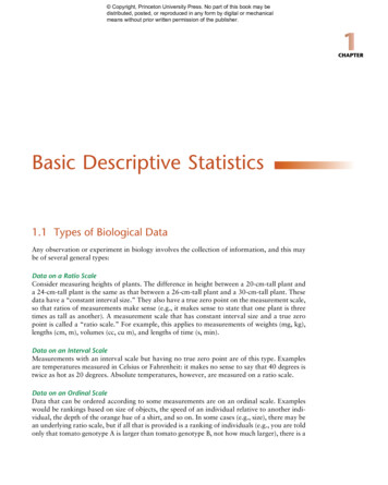
This is the R screen in Multiple-Document Interface (MDI) OTR6
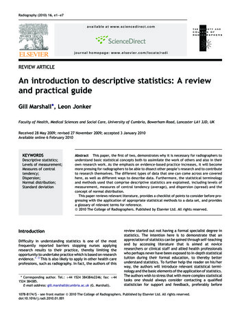
This is the R screen in Single-Document Interface (SDI) “ To make the SDI the default, you can select the SDI during installation of R, or edit the Rconsole configuration file in R's etc directory, changing the line MDI yes toMDI no. Alternatively, you can create a second desktop icon for R to run R in SDI mode: Make a copy of the R icon by right‐clicking on the icon and dragging it to a new location on the desktop. Release the mouse button and select Copy Here. Right‐click on the new icon and select Properties. Edit the Target field on the Shortcut tab to read "C:\Program Files\R\R‐2.5.1\bin\Rgui.exe" ‐‐sdi (including thequotes exactly as shown, and assuming that you've installed R to the default location). Then edit the shortcut name on the General tab to read something like R 2.5.1SDI . “ [John Fox, 1E/installation.html#SDI]OTR7
Working directorygetwd()# Shows the working directory (wd)setwd(choose.dir())# Select the working directory interactivelysetwd("C:/myfolder/data")# Changes the wdsetwd("H:\\myfolder\\data") # Changes the wdCreating directories/downloading from the internetdir()# Lists files in the working directorydir.create("C:/test")# Creates folder ‘test’ in drive ‘c:’setwd("C:/test")# Changes the working directory to “c:/test”# Download file ‘students.csv’ from the d "auto",quiet FALSE,mode "wb",cacheOK TRUE)OTR8
Installing/loading packages/user‐written programsinstall.packages("ABC")library(ABC)# This will install the package –-ABC--. A window will pop-up, select a# mirror site to download from (the closest to where you are) and click ok.# Load the package –-ABC-– to your workspace# Install the following rg/web/views/# Full list of packages by subject areaOperations/random numbers2 2Log(10)c(1, 1) c(1, 1)x - rnorm(10, mean 0, sd 1)xx - data.frame(x)x - matrix(x)# Creates 10 random numbers (normal dist.), syntax rnorm(n, mean, sd)OTR9
Keeping track of your work# Save the commands used during the sessionsavehistory(file "mylog.Rhistory")# Load the commands used in a previous sessionloadhistory(file "mylog.Rhistory")# Display the last 25 commandshistory()# You can read mylog.Rhistory with any word processor. Notice that the file has to have the extension*.RhistoryGetting help?plot # Get help for an object, in this case for the –-plot– function. You can also type: help(plot)?regression # Search the help pages for anything that has the word "regression". You can also type:help.search("regression")apropos("age")# Search the word "age" in the objects available in the current R session.help(package car)help(DataABC)args(log)# View documentation in package ‘car’. You can also type: library(help "car“)# Access codebook for a dataset called ‘DataABC’ in the package ABC# Description of the command.OTR10
Example of a dataset in Excel.Variables are arranged by columns and cases by rows. Each variable has more than one valuePath to the file: 1
From Excel to *.csvIn Excel go to File- Save as and save the Excel file as *.csv:You may get the following messages, click OK andYES OTR12
Data from *.csv (copy‐and‐paste)# Select the table from the excel file, copy, go to the R Console and type:mydata - read.table("clipboard", header TRUE, sep "\t")summary(mydata)edit(mydata)Data from *.csv (interactively)mydata - read.csv(file.choose(), header TRUE)Data from *.csvmydata - read.csv("c:\mydata\mydatafile.csv", header TRUE)mydata - ts.csv", header TRUE)Data from *.txt (space , tab, comma‐separated)# If you have spaces and missing data is coded as ‘-9’, type:mydata - read.table(("C:/myfolder/abc.txt", header TRUE, sep "\t", na.strings "-9")Data to *.txt (space , tab, comma‐separated)write.table(mydata, file "test.txt", sep "\t")OTR13
Data from Statainstall.packages("foreign")# Need to install package –-foreign–- first (you do this only once)library(foreign) # Load package –-foreign-mydata.stata - ts.dta")mydata.stata - .dta",convert.factors TRUE,convert.dates TRUE,convert.underscore TRUE,warn.missing.labels TRUE)# Where (source: type ?read.dta)# convert.dates. Convert Stata dates to Date class# convert.factors. Use Stata value labels to create factors? (version 6.0 or later).# convert.underscore. Convert " " in Stata variable names to "." in R names?# warn.missing.labels. Warn if a variable is specified with value labels and those value labels arenot present in the file.Data to Statawrite.dta(mydata, file "test.dta") # Direct export to Statawrite.foreign(mydata, codefile "test1.do", datafile "test1.raw", package "Stata") # Provide a dofile to read the *.raw dataOTR14
Data from SPSSinstall.packages("foreign")# Need to install package –-foreign–- first (you do this only once)library(foreign) # Load package –-foreign-mydata.spss - a.sav",to.data.frame TRUE,use.value.labels TRUE,use.missings to.data.frame)# Where:## ‘to.data.frame’ return a data frame.## ‘use.value.labels’ Convert variables with value labels into R factors with those levels.## ‘use.missings’ logical: should information on user-defined missing values be used to set thecorresponding values to NA.Source: type ?read.spssData to SPSS# Provides a syntax file (*.sps) to read the *.raw data filewrite.foreign(mydata, codefile "test2.sps", datafile "test2.raw", package “SPSS")OTR15
Data from SAS# To read SAS XPORT format (*.xpt). Package –-foreign-install.packages("foreign")# Need to install package –-foreign–- first (you do this only once)library(foreign) # Load package –-foreign-mydata.sas - read.xport("c:/myfolder/mydata.xpt") # NOTE: Does not work for files available online# Using package –-Hmisc—install.packages(“Hmisc")# Need to install package –-Hmisc–- first (you do this only once)library(Hmisc)mydata.sas - data.xpt")# It worksData to SAS# It provides a syntax file (*.sas) to read the *.raw datawrite.foreign(mydata, codefile "test2.sas", datafile "test2.raw", package “SAS")NOTE: As an alternative, you can use SAS Universal Viewer (freeware from SAS) to read SAS files and save them as *.csv. Saving the file as *.csvremoves variable/value labels, make sure you have the codebook available.OTR16
Data from ACII Record formmydata.dat -read.fwf(file th c(7, -16, 2, 2, -4, 2, -10, 2, -110, 3, -6, 2),col.names c("w","y","x1","x2","x3", "age", "sex"),n 1090)# Reading ASCII record form, numbers represent the width of variables, negative sign excludesvariables not wanted (you must include these).# To get the width of the variables you must have a codebook for the data set available (see anexample below).# To get the widths for unwanted spaces use the formula:Start of var(t 1) – End of var(t) - 1*Thank you to Scott Kostyshak for useful advice/code.Data locations usually available in 3var71OTR165166A217
Data from Rload("mydata.RData")load("mydata.rda")/* Add path to data if necessary */Data to Rsave.image("mywork.RData")# Saving all objects to file *.RDatasave(object1, object2, file “mywork.rda") # Saving selected objectsOTR18
Exploring datasummary(mydata)# Provides basic descriptive statistics and frequencies.edit(mydata)# Open data editorstr(mydata)# Provides the structure of the datasetnames(mydata)# Lists variables in the datasethead(mydata)# First 6 rows of datasethead(mydata, n 10)# First 10 rows of datasethead(mydata, n -10)tail(mydata)# All rows but the last 10# Last 6 rowstail(mydata, n 10)# Last 10 rowstail(mydata, n -10)# All rows but the first 10mydata[1:10, ]# First 10 rowsmydata[1:10,1:3] # First 10 rows of data of the first 3 variablesOTR19
Exploring the workspaceobjects()# Lists the objects in the workspacels()# Same as objects()remove()# Remove objects from the workspacerm(list ls())#clearing memory spacedetach(package:ABC)# Detached packages when no longer need themsearch()# Shows the loaded packageslibrary()# Shows the installed packagesdir()# show files in the working directoryOTR20
Missing datarowSums(is.na(mydata))# Number of missing per rowcolSums(is.na(mydata))# Number of missing per ta)# No. of missing per row (another way)# length num. of variables/elements in an object# Convert to missing datamydata[mydata age "&","age"] - NA# NOTE: Notice hidden spaces.mydata[mydata age 999,"age"] - NA# The function complete.cases() returns a logical vector indicating which cases are complete.# list rows of data that have missing valuesmydata[!complete.cases(mydata),]# The function na.omit() returns the object with listwise deletion of missing values.# Creating a new dataset without missing datamydata1 - na.omit(mydata)OTR21
Replacing a valuemydata1 - na.omit(mydata)mydata1[mydata1 SAT 1787,"SAT"] - 1800mydata1[mydata1 Country "Bulgaria","Country"] - "US"Renaming variables# Using base commandsfix(mydata)# Rename interactively.names(mydata)[3] - "First"# Using library –-reshape-library(reshape)mydata - rename(mydata, c(Last.Name "Last"))mydata - rename(mydata, c(First.Name "First"))mydata - rename(mydata, c(Student.Status "Status"))mydata - rename(mydata, c(Average.score.grade. "Score"))mydata - rename(mydata, c(Height.in. "Height"))mydata - rename(mydata, c(Newspaper.readership.times.wk. "Read"))OTR22
Value labels# Use factor() for nominal datamydata sex - factor(mydata sex, levels c(1,2), labels c("male", "female"))# Use ordered() for ordinal datamydata var2 - ordered(mydata var2, levels c(1,2,3,4), labels c("Strongly agree", "Somewhatagree", "Somewhat disagree", "Strongly disagree"))# As a new variable.mydata var8 - ordered(mydata var2, levels c(1,2,3,4), labels c("Strongly agree", "Somewhatagree", "Somewhat disagree", "Strongly disagree"))Reordering labelslevels(mydata Major)# Syntax for reorder(categorical variable, numeric variable, desired statistic)mydata Major with(mydata, reorder(Major,Read,mean))# Order goes from low to highlevels(mydata Major)attr(mydata Major, 'scores')# Reorder creates an attribute called ‘scores’ (with the statistic# used to reorder the labels, in this case the mean values.OTR# Mean of reading time: 4.4 for Econ, 5.3 for Math,4.9 for Politics (using students.xls)23
Creating ids/sequence of numbers# Creating a variable with a sequence of numbers or to index# Creating a variable with a sequence of numbers from 1 to n (where ‘n’ is the total number ofobservations)mydata id - seq(dim(mydata)[1])# Creating a variable with the total number of observationsmydata total - dim(mydata)[1]/* Creating a variable with a sequence of numbers from 1 to n per category (where ‘n’ is the totalnumber of observations in each category)(1) */mydata - mydata[order(mydata group),]idgroup - tapply(mydata group, mydata group, function(x) seq(1,length(x),1))mydata idgroup - unlist(idgroup)(1) Thanks to Alex Acs for the codeOTR24
Recoding variableslibrary(car)mydata Age.rec - recode(mydata Age, "18:19 '18to19';20:29 '20to29';30:39 '30to39'")mydata Age.rec - as.factor(mydata Age.rec)Sortmydata.sorted - mydata[order(mydata Gender),]mydata.sorted1 - mydata[order(mydata Gender, -mydata SAT),]Deleting variablesmydata Age.rec - NULLmydata var1 - mydata var2 - NULL(see subset next page)Deleting rows(see subset next page)OTR25
Subsetting variablesmydata2 - mydata[,1:14] # Selecting the first 14 variablesmydata2 - mydata[c(1:14)]sat - mydata[c("Last", "First", "SAT")]sat1 - mydata[c(2,3,11)]select - mydata[c(1:3, 12:14)]# Type names(select) to verifyselect1 - mydata[c(-(1:3), -(12:14))] # Excluding variablesSubsetting observationsmydata2 - mydata2[1:30,] # Selecting the first 30 observationsmydata3a - mydata[which(mydata Gender 'Female' & mydata SAT 1800), ]Subsetting variables/observationsmydata2 - mydata2[1:30,1:14]# Selecting the first 30 observations and first 14 variablesSubsetting using –subset‐‐mydata3mydata4mydata5mydata6 et(mydata2,Age 20 & Age Age 20 & Age Gender "Female" &Gender "Female" &30)30, select c(ID, First, Last, Age))Status "Graduate" & Age 30)Status "Graduate" & Age 30)OTR26
Categorical data: Frequencies/Crosstabstable(mydata Gender)table(mydata Read)# Two-way tablesreadgender - table(mydata Read,mydata Gender)readgenderaddmargins(readgender)# Adding row/col marginsprop.table(readgender,1)# Row proportionsround(prop.table(readgender,1), 2)# Round col prop to 2 digitsround(100*prop.table(readgender,1), 2)# Round col prop to 2 digits ), 2),2)# Round col prop to 2 digitsprop.table(readgender,2)# Column proportionsround(prop.table(readgender,2), 2)# Round column prop to 2 digitsround(100*prop.table(readgender,2), 2)# Round column prop to 2 digits ), 2),1)# Round col prop to 2 digitsprop.table(readgender)# Tot proportionsround(prop.table(readgender),2)# Tot proportions roundedround(100*prop.table(readgender),2)# Tot proportions adgender)# Do chisq test Ho: no relathionship# Do fisher'exact test Ho: no relationship# First two are assoc measures, last three show degree of association.# 3-way crosstabstable3 - xtabs( Read Major Gender, data mydata)table3ftable(table3a)# NOTE: Chi-sqr sum (obs-exp) 2/exp. Degrees of freedom for Chi-sqr are (r-1)*(c-1)OTR# NOTE: Chi-sqr contribution (obs-exp) 2/exp# Cramer's V sqrt(Chi-sqr/N*min). Where N is sample size and min is a the minimum of (r-1) or (c-1)27
Categorical data: Frequencies/Crosstabs using –gmodels‐‐library(gmodels)mydata ones - 1# Create a new variable of onesCrossTable(mydata Major,digits 2)# Shows horizontalCrossTable(mydata Major,digits 2, max.width 1)# Shows verticalCrossTable(mydata Major,mydata ones, digits 2)CrossTable(mydata Gender,mydata ones, digits 2)CrossTable(mydata Major,mydata Gender,digits 2, expected TRUE,dnn c("Major","Gender"))CrossTable(mydata Major,mydata Gender,digits 2, chisq TRUE, dnn c("Major","Gender"))CrossTable(mydata Major,mydata Gender,digits 2, dnn c("Major","Gender"))CrossTable(mydata Major,mydata Gender, format c("SPSS"), digits 1)chisq.test(mydata Major,mydata Gender)# Null hipothesis: no association# NOTE: Expected value (row total * column total)/overall total (or total sample size).Value we would expect if all cell were represented proportionally, whichindicates no association between variables. This is are we getting what weexpect or not. If so then nothing is new. If not then something is going onhttp://www.johndawes.com.au/page1/files/page1 apter 09 slides.pdf# NOTE: Chi-sqr sum (obs-exp) 2/expDegrees of freedom for Chi-sqr are (r-1)*(c-1)# NOTE: Chi-sqr contribution (obs-exp) 2/exp# Cramer's V sqrt(Chi-sqr/N*min)Where N is sample size and min is a the minimun of (r-1) or (c-1)OTR28
Measures of associationX2(chi‐square) tests for relationships between variables. The null hypothesis (Ho) is that there is no relationship. To reject this we need aPr 0.05 (at 95% confidence). Here both chi2 are significant. Therefore we conclude that there is some relationship betweenperceptions of the economy and gender. lrchi2 reads the same way.Cramer’s V is a measure of association between two nominal variables. It goes from 0 to 1 where 1 indicates strong association (for rXctables). In 2x2 tables, the range is ‐1 to 1. Here the V is 0.15, which shows a small association.Fisher’s exact test is used when there are very few cases in the cells (usually less than 5). It tests the relationship between two variables.The null is that variables are independent. Here we reject the null and conclude that there is some kind of relationship betweenvariablesSource: fPlotting lot(margin.table(readgender,2))OTR29
Descriptive Statistics using ","SAT","Score","Height", , basic TRUE, desc TRUE, norm TRUE, p 0.95)stat.desc(mydata[10:14], basic TRUE, desc TRUE, norm TRUE, p 0.95)OTR30
Descriptive Statisticsmean(mydata)# Mean of all numeric variablesmean(mydata SAT)with(mydata, mean(SAT))median(mydata SAT)var(mydata SAT)sd(mydata SAT)max(mydata SAT)min(mydata SAT)range(mydata SAT)quantile(mydata SAT)quantile(mydata SAT,fivenum(mydata SAT)# Variance# Standard deviation# Max value# Min value# Range# Quantiles 25%c(.3,.6,.9))# Customized quantiles# Boxplot elements. From help: "Returns Tukey's five number summary (minimum,# lower-hinge, median, upper-hinge, maximum) for the input data boxplot"length(mydata SAT)# Num of observations when a variable is specifylength(mydata)# Number of variables when a dataset is specifywhich.max(mydata SAT)# From help: "Determines the location, i.e., index of the (first) minimum or maximum of anumeric vector"which.min(mydata SAT)# From help: "Determines the location, i.e., index of the (first) minimum or maximum of anumeric vector”# Mode by frequenciestable(mydata Country)max(table(mydata Country))names(sort(-table(mydata Country)))[1]OTR31
Descriptive Statistics# Descriptive statistics by groups using --tapply--mean - tapply(mydata SAT,mydata Gender, mean) # Add na.rm TRUE to remove missing values in theestimationsd - tapply(mydata SAT,mydata Gender, sd)median - tapply(mydata SAT,mydata Gender, median)max - tapply(mydata SAT,mydata Gender, max)cbind(mean, median, sd, max)round(cbind(mean, median, sd, max),digits 1)t1 - round(cbind(mean, median, sd, max),digits 1)t1# Descriptive statistics by groups using --aggregate—aggregate(mydata[c("Age","SAT")],by list(sex mydata Gender), mean, na.rm er"], mean, na.rm TRUE)aggregate(mydata,by list(sex mydata Gender), mean, na.rm TRUE)aggregate(mydata,by list(sex mydata Gender, major mydata Major, status mydata Status), mean,na.rm TRUE)aggregate(mydata SAT,by list(sex mydata Gender, major mydata Major, status mydata Status), mean,na.rm TRUE)aggregate(mydata[c("SAT")],by list(sex mydata Gender, major mydata Major, status mydata Status),mean, na.rm TRUE)OTR32
Histogramslibrary(car)head(Prestige)hist(Prestige income)hist(Prestige income, col "green")with(Prestige, hist(income)) # Histogram of income with a nicer title.# Applying Freedman/Diaconis rule p.120 ("Algorithm that chooses bin widths and locationsautomatically, based on the sample size and the spread of the qucg6n.html)with(Prestige, hist(income, breaks "FD", col "green"))box()hist(Prestige income, breaks "FD")# Conditional histogramspar(mfrow c(1, 2))hist(mydata SAT[mydata Gender "Female"], breaks "FD", main "Female", xlab "SAT",col "green")hist(mydata SAT[mydata Gender "Male"], breaks "FD", main "Male", xlab "SAT", col "green")# Braces indicate a compound command allowing several commands with 'with' commandpar(mfrow c(1, 1))with(Prestige, {hist(income, breaks "FD", freq FALSE, col "green")lines(density(income), lwd 2)lines(density(income, adjust 0.5),lwd 1)rug(income)})OTR33
Histograms# Histograms overlaidhist(mydata SAT, breaks "FD", col "green")hist(mydata SAT[mydata Gender "Male"], breaks "FD", col "gray", add TRUE)legend("topright", c("Female","Male"), fill c("green","gray"))# Checksatgender - table(mydata SAT,mydata Gender)satgenderHistogram with normal curve overlayx - rnorm(100)hist(x, freq F)curve(dnorm(x), add(T)h - hist(x, plot F)ylim - range(0. h density, dnorm(0))hist(x, freq F, ylim ylim)curve(dnorm(x), add T)OTR34
Scatterplots# Scatterplots. Useful to 1) study the mean and variance functions in the regression of y on x p.128;2)to identify outliers and leverage points.# plot(x,y)plot(mydata SAT) # Index plotplot(mydata Age, mydata SAT)plot(mydata Age, mydata SAT, main “Age/SAT", xlab “Age", ylab “SAT", col "red")abline(lm(mydata SAT mydata Age), col "blue")# regression line (y x)lines(lowess(mydata Age, mydata SAT), col "green") # lowess line (x,y)identify(mydata Age, mydata SAT, row.names(mydata))# On row.names to identify. "All data frames have a row names attribute, a character vector of lengththe number of rows with no duplicates nor missing values." (source link below).# "Use attr(x, "row.names") if you need an integer value.)" tml/row.names.htmlmydata Names - paste(mydata Last, mydata First)row.names(mydata) - mydata Namesplot(mydata SAT, mydata Age)identify(mydata SAT, mydata Age, row.names(mydata))OTR35
Scatterplots# Rule on span for lowess, big sample smaller ( 0.3), small sample bigger ( 0.7)library(car)scatterplot(SAT Age, data mydata)scatterplot(SAT Age, id.method "identify", data mydata)scatterplot(SAT Age, id.method "identify", boxplots FALSE, data mydata)scatterplot(prestige income, span 0.6, lwd 3, id.n 4, data Prestige)# By groupsscatterplot(SAT Age Gender, data mydata)scatterplot(SAT Age Gender, id.method "identify", data mydata)scatterplot(prestige income type, boxplots FALSE, span 0.75, data Prestige)scatterplot(prestige income type, boxplots FALSE, span 0.75, col gray(c(0,0.5,0.7)), data Prestige)OTR36
Scatterplots (multiple)scatterplotMatrix( prestige income education women, span 0.7, id.n 0, data Prestige)pairs(Prestige)# Pariwise plots. Scatterplots of all variables in the datasetpairs(Prestige, gap 0, cex.labels 0.9) # gap controls the space between subplot and cex.labels thefont size (Dalgaard:186)3D Scatterplotslibrary(car)scatter3d(prestige income education, id.n 3, data Duncan)OTR37
Scatterplots (for categorical data)plot(vocabulary education, data Vocab)plot(jitter(vocabulary) jitter(education), data Vocab)plot(jitter(vocabulary, factor 2) jitter(education, factor 2), data Vocab)# cex makes the point half the size, p. 134plot(jitter(vocabulary, factor 2) jitter(education, factor 2), col "gray", cex 0.5, data Vocab)with(Vocab, {abline(lm(vocabulary education), lwd 3, lty "dashed")lines(lowess(education, vocabulary, f 0.2), lwd 3)})Useful links to graphicshttp://www.stat.auckland.ac.nz/ ques/thumbs.php?sort tmlOTR38
Exercises
Exercise 1Using the ICPSR Online Learning Center, go to guide on Civic Participation and Demographics in Rural China C/guides/China/sections/a01Got to the tab ‘Dataset’ and download the data des/China/sections/a02)We’ll focus on the first exercise on ‘Age and Participation’ and use the following variables: Respondent's year of birth (M1001)Village meeting attendance (M3090)Activities: Create the variable ‘age’ for each respondentCreate the variable ‘agegroup’ with the following categories: 16‐35, 36‐55 and 56‐79Questions: What percentage of respondents reported attending a local village meeting?Of those attending a meeting, which age group was most likely to report attending a village meeting?Of those attending a meeting , which group was most likely to report no village meeting attendance?Source: Inter‐university Consortium for Political and Social Research. Civic Participation and Demographics in Rural China: A Data‐DrivenLearning Guide. Ann Arbor, MI: Inter‐university Consortium for Political and Social Research [distributor], July, 31 2009.Doi:10.3886/ChinaOTR40
Exercise 2Got to the World Development Indicators (WDI) & Global Development Finance (GDF) from the World Bank (access from the library’sArticles and Databases, )Direct link to WDI/GDF http://databank.worldbank.org/ddp/home.do?Step 12&id 4&CNO 2Get data for the United States and all available years on: Long‐term unemployment (% of total unemployment)Long‐term unemployment, female (% of female unemployment)Long‐term unemployment, male (% of male unemployment)Inflation, consumer prices (annual %)GDP per capita (constant 2000 US )GDP per capita growth (annual %)See here to arrange the data as panel data df#page 21For an example of how panel data looks like click here: page 3Activities: Rename the variables and explore the data (use describe, summarize)Create a variable called crisis where it takes the value of 17 for the following years: 1960, 1961, 1969, 1970, 1973, 1974, 1975,1981, 1982, 1990, 1991, 2001, 2007, 2008, 2009. Replace missing with zeros (source: nber.org).Set as time series (see http://dss.princeton.edu/training/TS101.pdf#page 6)Create a line graph with unemployment rate (total, female and males) and crisis by year.Questions: What do you see? Who tends to be more affected by the economic recessions?OTR41
References/Useful links DSS Online Training Section http://dss.princeton.edu/training/ Princeton DSS Libguides http://libguides.princeton.edu/dss John Fox’s site http://socserv.mcmaster.ca/jfox/ Quick‐R http://www.statmethods.net/ UCLA Resources to learn and use R http://www.ats.ucla.edu/stat/R/ UCLA Resources to learn and use Stata http://www.ats.ucla.edu/stat/stata/ DSS ‐ Stata http://dss/online help/stats packages/stata/ DSS ‐ R http://dss.princeton.edu/online help/stats packages/rOTR42
References/Recommended books An R Companion to Applied Regression, Second Edition / John Fox , Sanford Weisberg, Sage Publications, 2011 Data Manipulation with R / Phil Spector, Springer, 2008 Applied Econometrics with R / Christian Kleiber, Achim Zeileis, Springer, 2008 Introductory Statistics with R / Peter Dalgaard, Springer, 2008 Complex Surveys. A guide to Analysis Using R / Thomas Lumley, Wiley, 2010 Applied Regression Analysis and Generalized Linear Models / John Fox, Sage, 2008 R for Stata Users / Robert A. Muenchen, Joseph Hilbe, Springer, 2010 Introduction to econometrics / James H. Stock, Mark W. Watson. 2nd ed., Boston: Pearson Addison Wesley,2007. Data analysis using regression and multilevel/hierarchical models / Andrew Gelman, Jennifer Hill. Cambridge ;New York : Cambridge University Press, 2007. Econometric analysis / William H. Greene. 6th ed., Upper Saddle River, N.J. : Prentice Hall, 2008. Designing Social Inquiry: Scientific Inference in Qualitative Research / Gary King, Robert O. Keohane, SidneyVerba, Princeton University Press, 1994. Unifying Political Methodology: The Likelihood Theory of Statistical Inference / Gary King, Cambridge UniversityPress, 1989 Statistical Analysis: an interdisciplinary introduction to univariate & multivariate methods / SamKachigan, New York : Radius Press, c1986 Statistics wi
# mirror site to download from (the closest to where you are) and click ok. library(ABC) # Load the package –-