Transcription
THE LITTLE BOOK OF GEOMORPHOLOGY:EXERCISING THE PRINCIPLE OF CONSERVATIONRobert S. Anderson
Table of Contents1. Introduction3General:2. The geotherm, permafrost and the lithosphere3. Gooshing of the mantle4. Climate system (energy)Inputs solar radiation patternRequired flux pattern to assure steady climate5. Cosmogenic radionuclides (atoms)Production, decay as source and sinkGeomorphic systems:6. Lakes (water volume)Sources, sinks and leaksSteady: what dictates the lake level?7. Continuity and a glacier surge8. Glaciers (ice volume)The steady pattern of ice discharge9. Weathering, production of radionuclide and pedogenic clay profiles (mineral)10. Hillslopes (regolith mass)Sources by weathering and by eolian depositionSinks by dissolutionWhat sets the steady shape of the hillslopeGilbert’s convex hilltops11. Groundwater12. Overland flow (water volume)Hortonian approximation13. Settling and unsettling14. Sediment transport (sediment volume)Spatial patterns of sediment discharge required at steady stateBedforms and the pattern of transport required15. River downstream fining (sediment concentration)Conservation of clasts of varying hardness/ erosion susceptibility16. Coastal littoral (sediment mass)What sets the pattern of longshore drift?How do grainsize and mineralogy evolve?17. MomentumSediment hop times18. Advection and the substantial derivative19. SummaryReferencesThe little book of 1221271301/7/08
1. IntroductionThere is no general theory of geomorphology. We cannot cast the subject in a singleequation, or set of equations. As with geology, geomorphology is a tangle of physics,chemistry, biology and history. It is also geometry, as the geomorphology plays out in acomplex geographic, topographic setting in which both the tectonic and climate processesresponsible for driving evolution of the topography change in style and intensity. Thereis no grand quest for a Universal Law of Geomorphology. Our subject is oftensubdivided according to the geographic elements of the geomorphic system: hillslopes,rivers, eolian dunes, glaciers, coasts, karst, and so on. You can see this in the chapters ofmost textbooks on geomorphology.That said, there is indeed order to the natural system on and near the earth’s surface thatin turn serves to connect these subdisciplines. Features in common among manygeomorphic realms include: Surface materials most often move in one direction: downhill, downstream, downdrift,or downwind. (Note that prior to emergence on the surface, the motion is effectivelyvertical, in the reference frame of the surface, during near-surface exhumation.) Materials are transformed as they move through the system. Some of this is againunidirectional, this time meaning irreversible: large grains can be broken into smallgrains, but not the reverse; chemical reactions are for the most part permanent, resultingin solutional loss and change in mineralogy toward low temperature hydrous phases.Exceptions to this general statement do exist: duricrusts form by cementation of soils, andcarbonate deposits accumulate. Motion is concentrative. Material gathers itself into more efficient streams (Shreve’sdichotomy of hillslopes and streams (Shreve, 1979)) resulting in spatially-branchingnetworks. This is one of several instances in which the surface processes lead to selforganization. If given enough time, the system evolves toward a state in which the material flow isadjusted to transport that supplied to it.These features argue for some degree of universality in our subject, some degree ofconnection between the elements of landscape and our treatment of those elements. Themost useful scientific principle that we will employ here is that of conservation:conservation of mass, of energy, and momentum. As Richard Feynman reminded us,keep track of the stuff in little boxes, and you can’t go wrong. The principles I refer tohere, and on which I dwell almost exclusively in this Little Book, are really derivatives ofthe statements that “mass is conserved” or “energy is conserved”. These are indeedfundamental laws of physics. And physicists lean on them heavily. So also ismomentum conserved, and angular momentum. So also is baryon number, strangeness,and so on. The fact that on the earth’s surface the speeds involved are far less than thespeed of light allows us to dodge the complexity introduced by Einstein; we can go rightback to Newton. As we do not need to worry about the conversion of mass to energy,mass is conserved perfectly.The little book of geomorphology31/7/08
Here is a general word statement capturing the essence of conservation:Rate of change of something rate of input – rate of loss /- sources or sinks of thatsomethingOf course, it is not always obvious what that “something” is in a particular problem. Ourfirst task is therefore to decide what to balance. For example, we must decide whether tocraft the balance for sediment mass or sediment volume, whether to balance the numberof radionuclides, or their concentration per unit volume. In addition, we must decidewhat region of the world we choose to craft this balance. Is it just a little 2D box? Is itwhole hillslope, is it a vertical pillar, or is it a 3D box across which this something mightbe transported across all sides? Formally, we are choosing the “control volume” for theproblem. We will see that these choices will depend on the system, and on the questionswe are asking of it.Our next task is to transform this word statement into a mathematical one. For the mostpart this follows easily if (and only if) we have been careful about setting up the wordproblem. The mathematical equations we derive will look quite similar, at least at somelevel. That this is the case allows us to make progress in solving them. While this is nota book about solving the problems in their most general form, I will work a few of thesimplest cases.The art comes in just how to set up the problems and as always with art, it is practicethat allows you to get better. This little book is aimed at providing that practice byshowing many examples of how to set up problems in quantitative geomorphology. Byassembling many examples between two covers not too widely spaced, I hope that youwill see the connections between the problems, and by seeing the connections be able toapproach new problems that are in one or another sense analogous to those I introduce onthese pages. We will see that the mathematics provides the bridge not only between thegeomorphic systems I discuss, but between our science and others – physics, from whichwe unabashedly borrow, but also chemistry and biology.The principle of conservation that I exercise here should serve the same purpose that themore fundamental laws of physics serve for the physicist. By being able to lean soheavily, or confidently, on these principles, we can cast our problems formally so that wecan then focus on what we do not know, and what we must know about the system inorder to make progress on it. My hope is that it will promote the formulation of bettergeomorphic experiments, and exploration of the world in search of the naturalexperiments.I realize that this all sounds fuzzy at the moment. Let me be more concrete. Themathematical statement that most frequently arises from writing down the statement ofconservation carefully sounds something like these words:The rate of change of some quantity at a site the spatial gradient in the rate of transportof that quantity the rate of birth of this quantity at the site - the rate of destruction at thesite.The little book of geomorphology41/7/08
Any progress beyond this point in the analysis of our system will then require that wecome to grips with what sets the transport rate (we need that before we can evaluate itsspatial gradient), and what sets the birth rate or rate of destruction (or death) of thequantity. As this still sounds a little fuzzy, let me illustrate with a biological example.Say our system is a band of sheep on a hillside in a mountain pasture (Figure 1). Foreconomic reasons we are interested only in live sheep. The sheep are wandering fromleft to right. The change of the number of sheep on the hillside, which we might measureby repeatedly photographing the hillside, will depend largely on the difference betweenthe number of sheep that leave the hillside to the right between times of measurement andthose that drift into the hillside from the left; any difference in these numbers will resultin accumulation or loss of sheep form the hillslope. But to this we must add any newlyborn lambs, and subtract any sheep that die (by whatever means – old age, coyotes,shepherds getting hungry). To make more progress than this, we would need moreknowledge about the biology of sheep. The rate of births, for example, should bedependent upon the concentration of ewes in the band (the rams are usually separatedfrom the ewes except in the breeding season). Prediction of the death rate would requireknowledge of the age structure of the band and some actuarial statistics for sheep. Itwould also involve the concentration of predators at the site, the number of coyotes orbears or wolves or eagles per unit area of landscape. So you see that by writing down theconservation equation we are automatically forced to focus on the other issues oftransport and of sources and sinks, in this case involving specific biological processes.I will take the ovine example one step further to ask a different question. Can we predict,instead of the number of sheep, the distribution of the ages of the sheep? In this case wemight alter the conservation equation to one in which we conserve sheep of each of manyage brackets. One would then have to account for the number of sheep that leave eachage class, by aging a year, the number of sheep that enter the age bracket by promotionfrom the next lower age bracket, and the number of sheep that die in each age bracket(the actuarial table again). We would end up with a set of equations that need to besolved, with explicit links between them. If we knew enough about sheep biology, wemight be able to predict the age structure of the band of sheep. Or, once we had carefullyformulated the set of equations, we could turn the question around and, given the agestructure of the band of sheep, determine some of these fundamental biological processes.The little book of geomorphology51/7/08
This is neither as far-fetched, nor as irrelevant to our quest as geomorphologists, as itmight sound. Biologists perform such an analysis all the time in order to understand andto model the demography of a population. To bring it back to geomorphology, thismethod is being exploited to modernize lichenometry (e.g., Loso et al., 2007). Theseauthors document the age distribution of a lichen population, from which they deduce therule set that controls the demography, really the population evolution, of lichen, which inturn is required before we make use of the distribution of lichen to deduce the age of thesurface on which they are growing.I have strayed into biological examples. But I hope you can see that the same strategycan be employed to organize our thoughts about what sets the size distribution of grainsin a river or along a coast, for example. Big grains can become little grains bycomminution (or breaking down), while little grains cannot stick themselves backtogether. Speaking mathematically, the big grains become a source for small grains andshow up as a source term in the conservation equation of little grains. Once smallenough, small grains may be lost from the system, as they get wafted out onto the shelffrom the beach system, or go into suspension and no longer participate in the shape orgrain size make-up of a river bed or a beach. We can organize these ideas and theprocesses they represent into conservation equations, again a linked set of equations, thatmust be simultaneously solved to predict the grainsize evolution of a system.Let me provide one more concrete example. Imagine that you are asked to assess theefficiency of a wood stove. You design a special room in which to place the wood stove,you load in some wood, and you light the fire. The room must be very well insulated, sothat the only way heat can enter or leave the room is through one inlet and one outlet.The little book of geomorphology61/7/08
Then you install measurement devices to monitor the heat that comes into the roomthrough the air inlet, the heat that leaves through the one outlet, the stovepipe, and thechange in the heat in the room itself. I think you would agree that the change in the heatin the room must be equivalent to the input of heat from the outside (through the inlet),minus the heat that leaves the room through the stovepipe, plus the heat produced by thestove (Figure 2). This is a statement of conservation of heat.The word picture is simply:Change of heat in the room input of heat from the outside – outlet of heat from theroom heat generated in the roomThe experiment I have described mirrors the manner in which the efficiency of variouswood stoves is actually measured. My first brush with the principle of conservation cameas an undergraduate student employed to help run such experiments designed by JayShelton, then a physics professor at Williams College (see Shelton and Shapiro (1976) fordescriptions of wood burning stoves and their proper operation). He simply turned theequation around to solve for the heat produced by the stove, placing all the measurablequantities on the right hand side of the equation:Heat generated in the room change of heat in the room – input of heat outlet of heatKnowing how much wood was placed in the stove (we weighed it), and its energy contentper unit mass (which depended upon its water content), we could then divide the heatproduced in the stove by the energy consumed to determine what fraction of the energywent into warming up the room.Efficiency heat generated in the room (by the stove) / heat content of the woodThe little book of geomorphology71/7/08
As an aside, one could place any heat source in the room. The most interesting exampleswere human beings, of which the college had many. It was through such experimentsthat Jay was able to determine that a typical college student, at rest, puts out energy at arate of about 100 Joules per second, or 100 watts. So if you ever need to know what youare worth as a producer of energy, think about a 100-watt light bulb.I have organized the book to move from general to geomorphic. I start with problemsthat are not purely geomorphic, but that are both pertinent and parallel in theirdevelopment. Two involve heat, and one introduces a dating method. I start with a heatproblem in which the conduction of heat dominates, a problem relevant to understandingthe temperature profile in the earth’s crust, which in turn is directly pertinent to thethickness of permafrost. But while I stop there with applications of the equations wederive (this is after all a Little Book), the same equation is the backbone to thinkingquantitatively about the variations in temperature to which near-surface rock and soil issubjected, which in turn influences the rates of chemical and mechanical breakdown ofrock. I then turn to another heat problem, the global climate system, in which the unevendistribution of radiation forces the world’s oceans and atmosphere to redistribute heatfrom the equatorial latitudes toward the poles. Next, the dating problem provides anexample of local sources and sinks, here the production of new nuclides from cosmicrays, and the decay of these nuclides to daughter products. This is the essence of manyatomic dating methods. The example provided is but a brief introduction to a blossomingfield of cosmogenic nuclide applications in the earth sciences. I introduce otherapplications in the weathering problem and in the coastal system.I then turn to geomorphic systems that will sound more familiar. I start with lakes, andask what combination of precipitation and evaporation sets a particular lake level. Thesection on glaciers deals with the expected pattern of ice discharge in a valley, and allowsus to predict the expected glacier length given a prescribed climate (by which here wemean the spatial pattern of local mass balance). I treat then the simplest case of in situweathering to predict the pattern of degree of weathering in a column of accumulatingsediment (e.g., loess or a floodplain). Here I take one baby step toward linking equationsfor different minerals: as the feldspars are the source of the clays, we must track theconcentrations of both. We then allow transport of the sediment by addressing theexpected shapes of a hillslope. Here we revisit the problem first worked by G. K. Gilbertto explain why hilltops are typically convex up. They are rounded, not spiky. I then pourwater (rain) on a hillside and ask what sets the spatial pattern of overland flow of wateron the slope. This is a prerequisite to answering how such an overland flow of watermight modify the landscape. Finally, I address two problems involving sedimenttransport. The first addresses what might form and allow the translation of bedforms likedunes and ripples. In the second, I go to the beach, and ask what sets the spatial patternof sediment transport (longshore drift) in the coastal or littoral zone.I summarize briefly by wrapping back to find the common thread among the problemstreated. While I do not solve all of the equations derived, I hint how one might go aboutexploring their behavior. Again, I emphasize that one can proceed in an organizedmanner, starting with steady solutions, 1D solutions, and proceeding to transient cases ofThe little book of geomorphology81/7/08
interest. Given that the thread I pull is a mathematical one, and that mathematics is ahighly evolved discipline with a long history of solving equations of the sort we derive,we can then borrow heavily on past experience in math and other fields that have alreadyaccessed this deep history.Finally, let me conclude this introduction with a caveat. This is not an encyclopedic bookon geomorphology. It cannot be so and remain small. It is meant as a tutorial on how toapproach geomorphic problems. There is not room to embellish by showing many realworld examples. We cannot even treat all of the geomorphic processes. I have left out,for example, the incision of bedrock by rivers, the formation of caves, the tectonicprocesses responsible for raising rock above sealevel, and so on. I am indeed working ona larger book to be published by Cambridge Press that will address all of these processes,titled Geomorphology: the Mechanics and Chemistry of Landscapes, co-authored withSuzanne Anderson. As this will be out soon, I needn’t apologize for the incompletenessof the little book you have before you. Think of it as an extended abstract in which I tryto capture the essence of our subject.Further readingFor examples of how analogous problems are set up in other fields, I recommend thefollowing textbooks.Turcotte and Schubert’s Geodynamics has for 20 years been a source of inspirationfor earth scientists. While they focus on geophysics, this has broadened in the mostrecent edition to include some geomorphic topics. But it is the geophysics, andparticularly the accessible treatment of heat and elastic problems that I most treasure.Carslaw and Jaeger’s Conduction of Heat in Solids is the bible on the topic of heattransport. It is something we all ought to have on our shelves for reference whenever aheat problem or something analogous to one (for example any diffusion problem) isapproached.Bird, Stewart, and Lightfoot’s Transport Phenomena, while targeted at engineers, is aclassic treatise on how to approach problems of heat and mass transport. The authorsprovide as well excellent atomic-level treatments of the origin of viscosity in fluids.Geoff Davies’s Dynamic Earth provides an avenue into thinking about the wholeearth as a system. As his aim is to explore the modes of motion in the earth’s mantle, hemust treat both thermal and fluid flow problems. These are intricately connected in theconvection process, either driven from the bottom, giving rise to plumes, or from the topfrom the sinking of cool slabs. He treats each of these problems at several levels, frombeginner to advanced.David Furbish, in his Fluid Physics in Geology: An Introduction to Fluid Motions onEarth's Surface and Within its Crust provides a formal introduction to many earth scienceproblems involving fluid flow. Many of these are geomorphic in character, but the bookis more general than that.Hornberger, Raffensperger, Wiberg and Eshelman, in their Elements of PhysicalHydrology, provide a well-illustrated, organized view of the hydrologic system. Theybegin many problems with a simple approach meant to develop the intuition of thereader.The little book of geomorphology91/7/08
John Harte’s Consider a Spherical Cow is a favorite for entrance into formaltreatment of environmental problems. The approach emphasizes scaling, and box modelsin which the principles of concern in this book are employed. I also have it on my shelffor its appendices, which like those in Turcotte and Schubert provide excellentsummaries of important physical constants and other “useful numbers”.I have also taken inspiration from Kerry Emanuel’s Divine Wind, a book about thescience and history of hurricanes. I appreciate the manner in which he has not shiedaway from talking about the science in some detail, and about how the science isaccomplished, in a book that is clearly targeted at a broad audience. He has also paidhomage to the art such events have inspired, through photography, poetry and prose. Ifind it a wonderful introduction to how the atmosphere works, as illuminated through thewindow of the most terrible storms. We need more such books.The little book of geomorphology101/7/08
2. The geotherm, permafrost and the lithosphereSorted circles, Spitzbergen. Naturally occurring self-organization of the beach sediment in the active layerabove permafrost. Coarse grains are sorted to the rims, leaving interior of the circles fine-grained. Scale ofcircles: roughly 2 m diameter.In this first chapter I ask what dictates the temperature profile within the earth’s crust.While this is not strictly geomorphology, it is an appropriate place to start because heatproblems serve as analogs for many other geomorphic problems, as we will see. Inaddition, knowledge of the temperature profile within the near-surface earth isfundamental to the interpretation of exhumation histories from thermochronology, for theprediction of the depth of permafrost, and may be used to deduce the temperature historyof the earth’s surface. Indeed, many near-surface processes are driven by changes intemperature, or have rates that are modulated by temperature. The rates of chemicalreactions, for example, are strongly dependent on temperature. This section is designed
to serve as an introduction to the basic physics of heat conduction in this region of theearth. It will serve as well as an introduction to diffusion problems.Consider the box depicted in Figure 1. This is called the control volume for the problem.While I have chosen a parallelepiped for its shape, with faces perpendicular to theCartesian coordinates x, y and z, I could have chosen any shape as long as it is a closedsurface. Our goal is to craft an equation for the evolution of temperature in the volume.We begin by writing an equation for the conservation of heat within this parcel of theearth. Here we take the material to be a solid, and do not allow it to be in motion(although this assumption could be relaxed later). The word picture for this statement ofconservation is:Rate of change of heat rate of heat input – rate of heat loss /- sources or sinks of heatEach term will have units of energy per unit time. The heat in the box is simply thetemperature of the box (which we can think of as the concentration of heat per unit mass),times the volume of the box, times the mass per unit volume (the density), times thethermal heat capacity (energy per unit mass per degree of temperature): H !cTdxdydz .The rate of change of this quantity with time is therefore the left hand side of thisequation. We use the partial derivative of the quantity with respect to time to represent!("cTdxdydz)the rate of change:, all other variables fixed, in other words, at a fixed!tpoint in space (x,y,z). Now we need an expression for the rate at which heat is comingacross the left hand side of the box. The heat moving across a boundary or wall of thebox can be written as the product of a heat flux, here denoted Q, with the area of the wall.The little book of geomorphology121/7/08
Throughout the book I will reserve the use of the term “flux” to mean the rate at whichsome quantity (here heat) moves per unit area per unit time. The inputs and losses ofheat across left and right walls will therefore look like Qxdxdz. The transport of heatacross the left wall is the product of Qx(x) (which reads “heat flux in the x-direction,evaluated at the location x”) with the area of the left wall, dy dz, while that crossing theright hand wall is the product of Qx(x dx), or the heat flux in the x direction evaluated atx dx with the area of the right wall, dy dz. Terms relating to the fluxes of heat across theother sides of the box are analogous. Our equation then becomes:! ( "cTdxdydz) Qx (x)dydz # Qx (x dx)dydz Qy (y)dxdz # Qy (y dy)dxdz(2.1)!t Qz (z)dxdy # Qz (z dz)dxdyUp to this point we have made very few assumptions. The only item missing is any heatthat is produced within the box, which could happen by radioactive decay of elements, orstrain heating of a fluid, or the change of phase of the material. We will ignore all ofthese for the present. Now let's simplify this a little. We can hold the volume of materialin this solid constant through time, allowing us to pull the dx, dy and dz out of the partialderivative with respect to time. For now I also assume that the density and the heatcapacity of the material do not change over the temperature range of interest. We maythen divide both sides by ρ c dx dy dz, and the equation simplifies to one of temperaturechange: 1 ' .0 *Qx (x dx) " Qx (x) ,- * Qy (y dy) " Qy (y) ,- * Qz (z dz) " Qz (z) ,- 20!T "& ) / 3 (2.2)!tdxdydz% #c ( 0140The last step involves the simple recognition that if we were to shrink the size of our boxso that dx tends toward zero, the terms in brackets on the right hand side are the spatialderivatives of the heat flux, !Qx /!x,!Qy /!y,!Qz /!z , and the final equation for theconservation of heat becomes 1 ' * !Q !Qy !Qz !T(2.3) "& ) x .!t!y!z /% #c ( , ! xIn doing this we are effectively using the definition of a derivative. This equation saysthat the temperature in a region will rise if there is a negative gradient in the flux of heatacross it, and vice versa (Figure 2). For example, if there is a positive gradient in the xdirection, then more heat is leaving out the right hand side of the box than is arrivingthrough the left hand side of the box, and the heat content and hence the temperature inthe box ought to decline.An alternative derivation using the Taylor series expansion. Before moving on, I want toshow you that we could have arrived at this equation by taking a slightly differentmathematical route. Back up to equation 3.1. We need expressions for the fluxes of heat,Q, at positions x dx, y dy and z dz. This time we will use a method of estimating thesevalues that employs what is known as a Taylor series expansion. As seen in Figure 3.2,the first estimate of Qx at x dx would be simply that at x, in other words Qx(x dx) Qx(x). A second, better estimate would entail projecting the slope of the function Q overthe distance dx. This would yield Qx(x dx) Qx (x) (dQx/dx * dx). You can see fromThe little book of geomorphology131/7/08
the figure that this ought to yield a better estimate. Better yet, you might take intoaccount the curvature of the function. A Taylor series expansion formalizes this processof estimation:!Q1 ! 2Q1 ! nQ2Q(x dx) Q(x) dx dx .(2.4)()( dx )n2n!x2 !xn! !xNote that as we take smaller and smaller elements, as we shrink our control volume, theterms with dx2, dx3 and so on, will become very small. These are called “higher orderterms”, and they may be neglected in the limit as dx- 0.Neglecting these higher order terms, when this estimate and the comparable ones forQy(y dy) and Qz(z dz) are inserted into equation 3.1, it becomes!Qy ' ! ( "cTdxdydz)!Qx ' Qx (x)dydz # & Qx (x) dx ) dydz Qy (y)dxdz # & Qy (y) dy dxdz%(%!t!x!y )(!Q ' Qz (z)dxdy # & Qz (z) z dz ) dxdy%!z ((2.5)Performing the subtractions yields!Qy!Q! ( "cTdxdydz)!Q # x dxdydz #dydxdz # z dzdxdy(2.6)!t!x!y!zDividing by ρcdxdydz, we arrive again at equation 3.3. The two mathematical routeshave converged at the same equation for conservation of heat.The little book of geomorphology141/7/08
We will from this point on assume that the heat problem is one-dimensional, and vertical.This will allow us to ignore gradients in heat flux in the horizontal dimensions. As wesee below, this situation arises when the gradients in temperature are small in thehorizontal relative to those in the vertical.As yet, we have not identified the specific process by which heat is transported in themedium. There are three means of heat transport: conduction, advection, and radiation.Radiation requires that the medium of concern is transparent in the proper wavelengths,which rock and soil certainly are not. Advection requires that the medium, or anotherfluid passing through it, be in motion. For now we are assuming that this is not the case.The principal means by which the near-surface rock is cooled is by conduction.Vibrat
The little book of geomorphology 3 1/7/08 1. Introduction There is no general theory of geomorphology. We cannot cast the subject in a single equation, or set of equations. As with geology, geomorphology is a tangle of physics, chemistry, biology and history.