WIXLIB

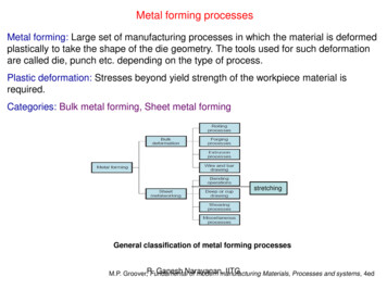
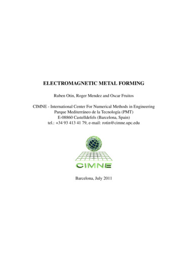
8CHAPTER 1. ELECTROMAGNETIC METAL FORMINGIn section 1.3.2 we explain how to compute the inductance Lcw (ω) and the resistance Rcw (ω)with the electromagnetic fields E(r, ω) and H(r, ω).In section 1.3.4 we show how to obtain the intensity I(t) with the calculated values of Lcw (ω)and Rcw (ω).Finally, in sections 1.3.5 and 1.3.6 we compute the Lorentz force acting on the workpiece withthe Fourier transform of I(t) and H(r, ω).Figure 1.1: RLC circuit used to produce the discharge current. In the shadowed rectangle at the left isrepresented the capacitor bank with capacitance Ccb , inductance Lcb and resistance Rcb . In the shadowedrectangle at the right is represented the system formed by the coil and the metal workpiece. This system hasan inductance Lcw and a resistance Rcw . Between both rectangles are represented the cables connectingthe capacitor bank with the coil. These cables have an inductance Lcon and a resistance Rcon .1.3.1Input dataThe input data required for computing the Lorentz force are:a) Geometry and material properties of the coil and the workpiece.b) Electrical parameters of the capacitor bank (capacitance Ccb , inductance Lcb , resistance Rcband initial voltage V0 ).c) Electrical parameters of the cables connecting the coil with the capacitor bank (inductanceLcon and resistance Rcon ).From the data in a) we calculate the inductance Lcw and the resistance Rcw of the system coilworkpiece as a function of the frequency ω. With Lcw (ω) and Rcw (ω) and the data in b) and c)

91.3. ELECTROMAGNETIC MODELwe find the intensity I(t) flowing through the RLC circuit of fig. 1.1. Finally, with I(t) and themagnetic field calculated with the data in a) we obtain the Lorentz force acting on the workpiece.In the following we analyze these steps in more detail.1.3.2Inductance and resistance of the system coil-workpieceThe repulsive force between the coil and the workpiece is a consequence of the time varyingcurrent I(t) generated in the RLC circuit of fig. 1.1. To calculate I(t) we first need the valuesof the inductance Lcw and the resistance Rcw . We do not take into account the capacitance ofthe system coil-workpiece because it is negligible in the geometries and at the frequencies usuallyinvolved in electromagnetic forming. The same is applicable to the capacitance of the cablesconnecting the coil with the capacitor bank.We consider the set coil-workpiece as a generic, two-terminal, linear, passive electromagneticsystem operating at low frequencies. We can imagine the coil and the workpiece inside a volumeυ with only its input terminals protruding. Under these assumptions, the inductance Lcw and theresistance Rcw at the frequency ω can be calculated with [11]Z1Lcw (ω) µ H(r, ω) 2 dυ,(1.1) In 2 υZ1Rcw (ω) σ E(r, ω) 2 dυ(1.2) In 2 υwhere In is the current injected into the system through the input terminals, µ is the magneticpermeability, H(r, ω) is the magnetic field, σ is the electrical conductivity and E(r, ω) is the electric field. The fields E(r, ω) and H(r, ω) are obtained after solving the time-harmonic Maxwell’sequations at a given frequency ω. For each frequency ω we have a different value of Lcw and Rcw .The injected current In is a dummy variable that is only used to drive the problem. It can take anyvalue without affecting the final result of (1.1) and (1.2).1.3.3Intensity in the RLC circuitIn fig. 1.1 is shown a typical RLC circuit used in electromagnetic forming. This circuit has aresistance R, an inductance L and a capacitance C given byR Rcb Rcon Rcw ,L Lcb Lcon Lcw ,(1.3)C Ccb .The values of R and L vary with time because of the deformation of the workpiece. In contrast, thecapacitance C remain constant during all the forming process. The intensity I(t) for all t [0, ]flowing through the circuit of fig. 1.1 satisfies the differential equation0 dd dI1(RI) (L ) I,dtdt dtC(1.4)

10CHAPTER 1. ELECTROMAGNETIC METAL FORMINGwith initial conditions V (t0 ) V0 and I(t0 ) 0. The initial value V0 represents the voltage atthe terminals of the capacitor. This voltage is related with the energy of the discharge U0 by1U0 CV02 .2(1.5)To find I(t) with (1.4) we have to know first R(t) and L(t) for all t [0, ].If we consider a loose coupling strategy, the functions R(t) and L(t) are constants and equal tothe values R0 and L0 calculated at the initial position with an un-deformed workpiece. Therefore,we have that R(t) R0 and L(t) L0 for all t [0, ]. Under these circumstances, the solutionof (1.4) is given byV0 γ0 tI(t) esin(ω0 t),(1.6)ω0 L0wheresω0 2πν0 andγ0 1 L0 C R02L0 2R0.2L0(1.7)(1.8)If we consider a sequential coupling strategy then we solve (1.4) in time intervals [ti , ti 1 ]. Thistime intervals correspond with the time periods between two successive calls to the electromagnetic equations. We can assume that L(t) and R(t) are constants inside each [ti , ti 1 ] and equalto the values Ri and Li calculated with the deformed workpiece at ti . In a sequential couplingstrategy , the expression (1.6) is the solution of the first time interval [t0 , t1 ].1.3.4Capacitance and frequencyEquation (1.6) shows that if we want to know the intensity I(t) we have to know first the valuesof ω0 , C, V0 , L0 and R0 . The capacitance C and the voltage V0 are given data. The inductance L0and the resistance R0 can be obtained with the help of (1.1), (1.2) and (1.3). The only value thatremains unknown is ω0 .The frequency ω0 is determined by the capacitance Ccb for a given set of coil, workpiece andconnectors. The frequency ω0 is the solution of the implicit equationC0 (ω) Ccb 0,(1.9)where the relation C0 (ω) is obtained after reordering expression (1.7)C0 (ω) 4L0 (ω).24ω L0 (ω)2 R0 (ω)2(1.10)In the case of using a sequential coupling strategy, we must take into account that the functionsLi (ω) and Ri (ω) are different in each [ti , ti 1 ] and, as a consequence, the frequency ωi is alsodifferent in each time interval.

111.3. ELECTROMAGNETIC MODEL1.3.5Lorentz force on the workpieceTo calculate the electromagnetic force acting on the workpiece we made the following assumptions:i) The dimensions of the system coil-workpiece are small compared with the wavelength ofthe prescribed fields. The wavelengths involved in EMF are in the order of λ 103 105 mwith frequencies in the order of ν 103 104 Hz. As a consequence of this, we canconsider the displacement current negligible D/ t 0 and to treat the fields as if theypropagated instantaneously with no appreciable radiation [23, 11].ii) The workpiece is linear, isotropic, homogeneous and non-magnetic (µ µ0 ). These properties represent all the workpieces used in this work (aluminium alloys). If we want to consider more complex materials, we must add to (1.11) the surface and volumetric integralsdescribed in [23].iii) The modulus of the velocity at any point in the workpiece is always much less than v 107 m/s. In fact, the velocities involved in EMF are in the order of v 102 103 m/s. Thiscircumstance allows us to neglect the velocity terms that appear in the Maxwell’s equationswhen working with moving media [15].Under hypothesis i)-iii) we can express the total force acting on the workpiece by [16]ZZF fυ dυ (J B) dυ,υ(1.11)υwhere fυ is a volumetric force density, J σE is the current density induced in the workpieceand B µ0 H is the magnetic flux density. If we use the vector identity 1B B B 2 (B · ) B,(1.12)2and recalling that, by hypothesis i) and ii), the Ampere’s circuital law is B µ0 J,(1.13)we can write the force density fυ as fυ 1 B 22µ0 1(B · ) B.µ0(1.14)In EMF the last term of the right hand side is usually negligible compared with the first. This is sobecause the field B is almost unidirectional in the area of the workpiece just in front of the coil.In this area is where the main contribution to the total force is produced and also where the highervalues of the Lorentz force are found. If a field B is unidirectional then, by the Gauss law formagnetism ( · B 0), it will not change in the direction of B. If a field B only changes in thedirections perpendiculars to B then we have that (B · ) B 0. In other words, to neglect the

12CHAPTER 1. ELECTROMAGNETIC METAL FORMINGlast term of (1.14) is equivalent to neglect the compressive and expansive forces parallels to theworkpiece surface and to state that, in EMF, the Lorentz force is due to the change in magnitudeof the magnetic field along the thickness of the workpiece. Therefore, in EMF, we can simplify(1.14) to 12fυ (1.15) B .2µ0Sometimes, the computational codes that solve the mechanical equations work more easily withpressures than with volumetric forces densities. In such cases, it is advantageous to express theforce acting on the workpiece as a magnetic pressure applied on its surface. This magnetic pressureis the line integral of (1.15) from a point r0 placed on the workpiece surface nearest to the coil toa point rτ placed on the opposite side of the workpiece. The path to follow is a straight line witha direction defined by the surface normal at r0 . The magnetic pressure is then given byZ rτ 1fυ ds P (r0 , t) B(r0 , t) 2 B(rτ , t) 2 ,(1.16)2µ0r0which it can be also expressed as a function of H recalling that, by hypothesis (ii), B µ0 HP (r0 , t) 1µ0 H(r0 , t) 2 H(rτ , t) 2 .2(1.17)We can conclude from equation (1.17) that, under hypothesis i)-iii), we only need to know H(r, t) on the surfaces of the workpiece to characterize electromagnetically the EMF process.1.3.6Lorentz force in frequency domainThe fields H(r, t) of (1.17) can be represented in frequency domain using the inverse Fouriertransform as followsZ 1H(r, t) [Hn (r, ω) I(ω)] eiωt dω,(1.18)2π where i 1 is the imaginary unit, Hn (r, ω) is the magnetic field per unit intensity at thefrequency ω and I(ω) is the Fourier transform of the intensity I(t) flowing through the RLCcircuitZ I(ω) I(t) e iωt dt.(1.19) If the intensity I(t) is given by (1.6) then the analytical expression of I(ω) is 111I(ω) ,2 ω ω0 iγ0 ω ω0 iγ0(1.20)where ω0 is the frequency (1.7) and γ0 is defined in (1.8). The magnetic field per unit intensityHn (r, ω) is defined byH(r, ω)Hn (r, ω) ,(1.21)Inwhere H(r, ω) and In are the same magnetic field and intensity as the ones appearing in (1.1).

1.4. NUMERICAL ANALYSIS TOOLS13We can write the Fourier transform of H(r, t) as it is shown in (1.18) because, by hypothesisi) and ii), we are in the quasi-static regime and in the presence of linear materials. This impliesthat the magnetic field has almost a constant phase inside the system coil-workpiece and thatit is linearly related with the current intensity. Also, it implies that the magnetic field and thecurrent are in phase and, as a consequence, Hn (r, ω) is approximately a real number Hn (r, ω) Real [Hn (r, ω)]. The advantage of using Hn (r, ω) is that we can know the magnetic field insidethe system coil-workpiece for any value of the current intensity I(ω) once it is known for In .1.4Numerical analysis toolsTwo different numerical tools are used to simulate the electromagnetic forming process. Onesolves the electromagnetic equations and the other solves the mechanical equations. The inputdata a)-c) (section 1.3.1) are provided to the electromagnetic code to obtain the magnetic pressure(1.17) on the surfaces of the workpiece. Afterwards, this magnetic pressure is provided to themechanical code to obtain the deformation workpiece.The electromagnetic equations are solved with the in-house code ERMES. The numericalformulation behind ERMES is explained in detail in [18].The mechanical equations are solved with the commercial software STAMPACK [22]. Thisnumerical tool has been applied to processes such as ironing, necking, embossing, stretch-forming,forming of thick sheets, flex-forming, hydro-forming, stretch-bending of profiles, etc. It can solvedynamic problems with high speeds and large strains rates, obtaining explicitly accelerations,velocities and deformations. In this work, our emphasis is on the electromagnetic part of the EMFprocess, then, we do not go further into the numerical formulation behind STAMPACK. For adetailed information about this formulation see [3].1.5Application example I. Sheet bulging.In this section we apply the electromagnetic model explained above to the EMF process presentedin [25]. This process consists in the free bulging of a thin metal sheet by a spiral flat coil. Ourobjective is to find the magnetic pressure acting on the workpiece for the given value of the capacitance Ccb 40 µF and the initial voltage V0 6 kV.1.5.1Description of the system coil-workpieceThe spiral flat coil appearing in [25] can be approximated by coaxial loop currents in a plane. Thus,the problem can be considered axis symmetric. The dimensions of the coil and the workpiece areshown in fig. 1.2. The diameter of the wire, material properties and horizontal positioning of thecoil are missed in [25]. We used the values given in [7], where the same problem is treated and itis provided a complete description of the geometry.The coil is made of copper with an electrical conductivity of σ 58e6 S/m. The workpiece isa circular plate of annealed aluminum JIS A 1050 with an electrical conductivity of σ 36e6 S/m.

14CHAPTER 1. ELECTROMAGNETIC METAL FORMINGIt is assumed 0 and µ µ0 in the coil and in the workpiece.The RLC circuit has an inductance Lcb Lcon 2.0 µH, a resistance Rcb Rcon 25.5 mΩand a capacitance Ccb 40 µF. The capacitor bank was initially charged with a voltage of V0 6 kV.Figure 1.2: Dimensions of the system coil-workpiece. Data taken from [25, 7]. Number of turns of the coilN 5. Pitch or coil separation p 5.5 mm. Diameter of the coil wires d 1.29 mm (16 AWG). Maximumcoil radius rext 32 mm. Minimum coil radius rint 8.71 mm. Separation distance between coil andmetal sheet h 1.6 mm. Thickness of the sheet τ 0.5 mm. Radius of the workpiece Rwp 55 mm.1.5.2Finite element modelAlthough, undoubtedly, in this case the best option is to perform the computations with an axissymmetric two-dimensional computational tool, we used the in-house three-dimensional code ERMES. The advantages are that we do not need to build a new tool and that we can solve moregeneral situations with the same software and the same file exchange interface between ERMESand STAMPACK. On the other hand, for this specific problem, our tools are computationally lessefficient.We employed the geometry shown in fig. 1.3 to compute the electromagnetic fields withERMES. The geometry is a truncated portion of a sphere with an angle of 20o . We drive theproblem with a current density J uniformly distributed in the volume of the coil wires. In thecolored surfaces of fig. 1.3 we imposed the regularized perfect electric conductor (PEC) boundaryconditions (see chapter 3) · (εE) 0,n̂ E 0.(1.22)It is not necessary to impose more boundary condition if we apply in all the FEM nodes of thedomain a change of coordinates from cartesian (Ex , Ey , Ez ) to axis symmetric around the Y axis(Eρ , Eϕ , Ey ). That is, at the same time we are building the matrix, we enforce at each node of the

1.5. APPLICATION EXAMPLE I. SHEET BULGING.15FEM mesh the following Eρx/ρ 0 z/ρEx Eϕ z/ρ 0 x/ρ Ey Ey01 0Ez(1.23) where x and z are the cartesian coordinates of the node and ρ x2 z 2 . We preserve thesymmetry of the final FEM matrix applying (1.23) and its transpose as it is explained in [2].The advantage of using (1.23) is that Eρ 0 and Ey 0 in axis symmetric problems. Thisfact reduces by a factor of three the size of the final matrix and also the time required to solveit. Therefore, we can improved noticeably the computational performance of ERMES in axissymmetric problems with a simple modification of its matrix building procedure. In a desktopcomputer with a CPU Intel Core 2 Quad Q9300 at 2.5 GHz and the operative system MicrosoftWindows XP, ERMES requires less than 30 s and less than 500 MB of memory RAM to solveeach frequency.Figure 1.3: Geometry used in ERMES to compute the electromagnetic fields in the free bulging process ofa thin metal sheet by a spiral flat coil.

16CHAPTER 1. ELECTROMAGNETIC METAL FORMING1.5.3Intensity through the RLC circuitOnce the initial geometry of system coil-workpiece is properly characterized, we have to find theintensity I(t) flowing through the RLC circuit. As it is mentioned in section 1.3.4, if we wantto know I(t) we have to calculate first the frequency ω0 . This frequency ω0 is the solution ofequation (1.9) with Ccb 40 µF. We solved (1.9) using the following iterative procedure:1) We replace in C0 (ω) the frequency which satisfies δ τ , where τ is the thickness of theworkpiece and δ is the skin depthr1δ .(1.24)πνµσ2) We compare C0 (ω) with Ccb . If C0 (ω) Ccb then we must increase the value of ω. IfC0 (ω) Ccb then we must decrease the value of ω. If C0 (ω) Ccb then we have foundthe solution ω0 .3) If the solution is not achieved then we replace in C0 (ω) the new incremented/decrementedvalue of ω and go to step 2). The procedure is repeated until the solution is achieved.In fig. 1.4 is shown the capacitance C0 as a function of the frequency ν and the solution ν0 16.35 kHz for the given capacitance Ccb 40 µF. We have choose an initial frequency satisfyingδ τ because we have observed in the literature that the typical frequencies employed in EMFlay in the intervalδ0.5 1.5.(1.25)τIn the present case, we have that the skin depth is δ 1.3 τ .As it is indicated in equation (1.10), we need to know L0 (ω) and R0 (ω) to calculate C0 (ω).These functions are defined in (1.3) and they represent the total inductance and the total resistanceof the RLC circuit of fig. 1.1. We assume that the given values Lcb Lcon 2.0 µH andRcb Rcon 25.5 mΩ do not change with the frequency. On the other hand, Lwp and Rwp arefrequency dependant and they have to be calculated with the help of (1.1) and (1.2). In the volumeof the coil, equation (1.2) is replaced byZ1 J 2Rcw (ω) dυ(1.26)2 In υ σwhere J is the imposed current density and σ is the conductivity of the coil. We recall that if wewant to obtain a volume integral for all the space then we must multiply by 18 ( 360o /20o ) anyvolume integral calculated in

Electromagnetic metal forming This report presents a numerical model for computing the Lorentz force that drives an electromag-netic forming process. This model is also able to estimate the optimum capacitance at which it is attained the maximum workpiece