Transcription
Real Business Cycle Models:Past, Present, and Future Sergio Rebelo†March 2005AbstractIn this paper I review the contribution of real business cycles modelsto our understanding of economic fluctuations, and discuss open issues inbusiness cycle research. I thank Martin Eichenbaum, Nir Jaimovich, Bob King, and Per Krusell for their comments,Lyndon Moore and Yuliya Meshcheryakova for research assistance, and the National ScienceFoundation for financial support.†Northwestern University, NBER, and CEPR.
1. IntroductionFinn Kydland and Edward Prescott introduced not one, but three, revolutionaryideas in their 1982 paper, “Time to Build and Aggregate Fluctuations.” The firstidea, which builds on prior work by Lucas and Prescott (1971), is that businesscycles can be studied using dynamic general equilibrium models. These modelsfeature atomistic agents who operate in competitive markets and form rationalexpectations about the future. The second idea is that it is possible to unifybusiness cycle and growth theory by insisting that business cycle models must beconsistent with the empirical regularities of long-run growth. The third idea isthat we can go way beyond the qualitative comparison of model properties withstylized facts that dominated theoretical work on macroeconomics until 1982.We can calibrate models with parameters drawn, to the extent possible, frommicroeconomic studies and long-run properties of the economy, and we can usethese calibrated models to generate artificial data that we can compare with actualdata.It is not surprising that a paper with so many new ideas has shaped themacroeconomics research agenda of the last two decades. The wave of models thatfirst followed Kydland and Prescott’s (1982) work were referred to as “real businesscycle” models because of their emphasis on the role of real shocks, particularlytechnology shocks, in driving business fluctuations. But real business cyle (RBC)models also became a point of departure for many theories in which technologyshocks do not play a central role.In addition, RBC-based models came to be widely used as laboratories forpolicy analysis in general and for the study of optimal fiscal and monetary policy in particular.1 These policy applications reflected the fact that RBC models1See Chari and Kehoe (1999) for a review of the literature on optimal fiscal and monetarypolicy in RBC models.2
represented an important step in meeting the challenge laid out by Robert Lucas(Lucas (1980)) when he wrote that “One of the functions of theoretical economicsis to provide fully articulated, artificial economic systems that can serve as laboratories in which policies that would be prohibitively expensive to experiment within actual economies can be tested out at much lower cost. [.] Our task as I seeit [.] is to write a FORTRAN program that will accept specific economic policyrules as ‘input’ and will generate as ‘output’ statistics describing the operatingcharacteristics of time series we care about, which are predicted to result fromthese policies.”In the next section I briefly review the properties of RBC models. It wouldhave been easy to extend this review into a full-blown survey of the literature. ButI resist this temptation for two reasons. First, King and Rebelo (1999) alreadycontains a discussion of the RBC literature. Second, and more important, thebest way to celebrate RBC models is not to revel in their past, but to considertheir future. So I devote section III to some of the challenges that face the theoryedifice that has built up on the foundations laid by Kydland and Prescott in 1982.Section IV concludes.2. Real Business CyclesKydland and Prescott (1982) judge their model by its ability to replicate themain statistical features of U.S. business cycles. These features are summarizedin Hodrick and Prescott (1980) and are revisited in Kydland and Prescott (1990).Hodrick and Prescott detrend U.S. macro time series with what became known asthe “HP filter.” They then compute standard deviations, correlations, and serialcorrelations of the major macroeconomic aggregates.Macroeconomists know their main findings by heart. Investment is about threetimes more volatile than output, and nondurables consumption is less volatile3
than output. Total hours worked and output have similar volatility. Almost allmacroeconomic variables are strongly procyclical, i.e. they show a strong contemporaneous correlation with output.2 Finally, macroeconomic variables showsubstantial persistence. If output is high relative to trend in this quarter, it islikely to continue above trend in the next quarter.Kydland and Prescott (1982) find that simulated data from their model showthe same patterns of volatility, persistence, and comovement as are present inU.S. data. This finding is particularly surprising, because the model abstractsfrom monetary policy, which economists such as Friedman (1968) consider animportant element of business fluctuations.Instead of reproducing the familiar table of standard deviations and correlations based on simulated data, I adopt an alternative strategy to illustrate theperformance of a basic RBC model. This strategy is similar to that used by theBusiness Cycle Dating Committee of the National Bureau of Economic Research(NBER) to compare different recessions (see Hall et al. (2003)) and to the methods used by Burns and Mitchell (1946) in their pioneer study of the properties ofU.S. business cycles.I start by simulating the model studied in King, Plosser, and Rebelo (1988) for5,000 periods, using the calibration in Table 2, column 4 of that paper. This modelis a simplified version of Kydland and Prescott (1982). It eliminates features thatare not central to their main results: time-to-build in investment, non-separableutility in leisure, and technology shocks that include both a permanent and atransitory component. I detrend the simulated data with the HP filter. I identifyrecessions as periods in which output is below the HP trend for at least threeconsecutive quarters.32A notable exception is the trade balance which is countercyclical. See Baxter and Crucinni(1993).3Interestingly, applying this method to U.S. data produces recession dates that are similar to4
Figure 1 shows the average recession generated by the model. All variables arerepresented as deviations from their value in the quarter in which the recessionstarts, which I call period zero. This figure shows that the model reproduces thefirst-order features of U.S. business cycles. Consumption, investment, and hoursworked are all procyclical. Consumption is less volatile than output, investmentis much more volatile than output, and hours worked are only slightly less volatilethan output. All variables are persistent. One new piece of information I obtainfrom Figure 1 is that recessions in the model last for about one year, just as inthe U.S. data.3. Open Questions in Business Cycle ResearchI begin by briefly noting two well-known challenges to RBC models. The first isexplaining the behavior of asset prices. The second is understanding the GreatDepression. I then discuss research on the causes of business cycles, the role oflabor markets, and on explanations for the strong patterns of comovement acrossdifferent industries.The Behavior of Asset Prices Real business cycle models are arguably successful at mimicking the cyclical behavior of macroeconomic quantities. However,Mehra and Prescott (1985) show that utility specifications common in RBC models have counterfactual implications for asset prices. These utility specificationsare not consistent with the difference between the average return to stocks andthose chosen by the NBER dating committee. The NBER dates for the beginning of a recessionand the dates obtained with the HP procedure (indicated in parentheses) are as follows: 1948IV (1949-I), 1953-II (1953-IV), 1960-II (1960-III), 1969-IV (1970-I), 1973-III (1974-III), 1981-III(1981-IV), 1990-III (1990-IV), and 2001-I (2001-III). The NBER dates include 1980-I, whichis not selected by the HP procedure. In addition, the HP procedure includes three additionalrecessions starting in 1962-III, 1986-IV, 1995-I. None of the latter episodes involved a fall inoutput.5
bonds. This “equity premium puzzle” has generated a voluminous literature, recently reviewed by Mehra and Prescott (2003).Although a generally accepted resolution of the equity premium puzzle is currently not available, many researchers view the introduction of habit formationas an important step in addressing some of the first-order dimensions of the puzzle. Lucas (1978)-style endowment models, in which preferences feature simpleforms of habit formation, are consistent with the difference in average returnsbetween stocks and bonds. However, these models generate bond yields that aretoo volatile relative to the data.4Boldrin, Christiano, and Fisher (2001) show that simply introducing habitformation into a standard RBC model does not resolve the equity premium puzzle. Fluctuations in the returns to equity are very small, because the supply ofcapital is infinitely elastic. Habit formation introduces a strong desire for smoothconsumption paths, but these smooth paths can be achieved without generatingfluctuations in equity returns. Boldrin, et al. (2001) modify the basic RBC modelto reduce the elasticity of capital supply. In their model investment and consumption goods are produced in different sectors and there are frictions to thereallocation of capital and labor across sectors. As a result, the desire for smoothconsumption introduced by habit formation generates volatile equity returns anda large equity premium.What Caused the Great Depression? The Great Depression was the mostimportant macroeconomic event of the 20th century. Many economists interpretthe large output decline, stock market crash, and financial crisis that occurredbetween 1929 and 1933 as a massive failure of market forces that could have been4Early proponents of habit formation as a solution to the equity premium puzzle includeSundaresan (1989), Constantinides (1990), and Abel (1990). See Campbell and Cochrane (1999)for a recent discussion of the role of habit formation in consumption-based asset pricing models.6
prevented had the government played a larger role in the economy. The dramaticincrease in government spending as a fraction of GDP that we have seen since the1930s is partly a policy response to the Great Depression.In retrospect, it seems plausible that the Great Depression resulted from anunusual combination of bad shocks compounded by bad policy. The list of shocksincludes large drops in the world price of agricultural goods, instability in thefinancial system, and the worst drought ever recorded. Bad policy was in abundantsupply. The central bank failed to serve as lender of last resort as bank runs forcedmany U.S. banks to close. Monetary policy was contractionary in the midst ofthe recession. The Smoot-Hawley tariff of 1930, introduced to protect farmersfrom declines in world agricultural prices, sparked a bitter tariff war that crippledinternational trade. The federal government introduced a massive tax increasethrough the Revenue Act of 1932. Competition in both product and labor marketswas undermined by government policies that permitted industry to collude andincreased the bargaining power of unions. Using rudimentary data sources to sortout the effects of these different shocks and different policies is a daunting task,but significant progress is being made.5What Causes Business Cycles? One of the most difficult questions in macroeconomics asks, what are the shocks that cause business fluctuations? Longstanding suspects are monetary, fiscal, and oil price shocks. To this list Prescott(1986) adds technology shocks, and argues that they “account for more than halfthe fluctuations in the postwar period with a best point estimate near 75%”.The idea that technology shocks are the central driver of business cycles is controversial. Prescott (1986) computes total factor productivity (TFP) and treatsit as a measure of exogenous technology shocks. However, there are reasons to5See Christiano, Motto, and Rostagno (2005), Cole and Ohanian (1999, 2004), and theJanuary 2002 issue of the Review of Economic Dynamics and the references therein.7
distrust TFP as a measure of true shocks to technology. TFP can be forecast using military spending (Hall (1988)), or monetary policy indicators (Evans (1992)),both of which are variables that are unlikely to affect the rate of technical progress.This evidence suggests that TFP, as computed by Prescott, is not a pure exogenous shock, but has some endogenous components. Variable capital utilization,considered by Basu (1996) and Burnside, Eichenbaum, and Rebelo (1996); variability in labor effort, considered by Burnside, Eichenbaum, and Rebelo (1993);and changes in markup rates, considered by Jaimovich (2004a), drive importantwedges between TFP and true technology shocks. These wedges imply that themagnitude of true technology shocks is likely to be much smaller than that of theTFP shocks used by Prescott.Burnside and Eichenbaum (1996), King and Rebelo (1999), and Jaimovich(2004a) argue that the fact that true technology shocks are smaller than TFPshocks does not imply that technology shocks are unimportant. Introducing mechanisms such as capacity utilization and markup variation in RBC models has twoeffects. First, these mechanisms make true technology shocks less volatile thanTFP. Second, they significantly amplify the effects of technology shocks. Thisamplification allows models with these mechanisms to generate output volatilitysimilar to the data with much smaller technology shocks.Another controversial aspect of RBC models is the role of technology shocksin generating recessions. The NBER business cycle dating committee defines arecession as “a significant decline in economic activity spread across the economy,lasting more th
Real Business Cycle Models: . Kydland and Prescott (1982) find that simulated data from their model show the same patterns of volatility, persistence, and comovement as are present in U.S. data. This finding is particularly surprising, because the model abstracts from monetary policy, which economists such as Friedman (1968) consider an important element of business fluctuations. Instead .
