WIXLIB

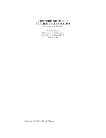
LECTURE 1. INTRODUCTION5When dimensionless parameters exist, we have a choice in how we define dimensionless variables. For example, on a finite domain, we could nondimensionalize asabove, which would give (1.8) on a domain of length R. Alternatively, we mightprefer to use the length of the domain to nondimensionalize lengths. In that case,the nondimensionalized domain has length 1, and the nondimensionalized form of(1.5) is1ut uxx u (1 u) .RWe get a small, or large, dimensionless diffusivity if the diffusive timescale is large,or small, respectively, compared with the reaction time scale.Somewhat less obviously, even on infinite domains additional lengthscales maybe introduced into a problem by initial datau(x, 0) u0 (x).Using the variables (1.7), we get the nondimensionalized initial conditionū (x̄, 0) ū0 (x̄) ,where1u0 (Lx̄) .aThus, for example, if u0 has a typical amplitude a and varies over a typical lengthscale of , then we may write x u0 (x) af where f is a dimensionless function. Then ū0 (x̄) f Rx̄ ,ū0 (x̄) and the evolution of the solution depends upon whether the initial data variesrapidly, slowly, or on the same scale as the reaction-diffusion length scale L.3.5. Traveling wavesOne of the principal features of the KPP equation is the existence of traveling waveswhich describe the invasion of an unpopulated region (or a region whose populationdoes not possess the favorable allele) from an adjacent populated region.A traveling wave is a solution of the form(1.9)u(x, t) f (x ct)where c is a constant wave speed. This solution consists of a fixed spatial profilethat propagates with velocity c without changing its shape.For definiteness we assume that c 0. The case c 0 can be reduced tothis one by a reflection x 7 x, which transforms a right-moving wave into aleft-moving wave.Use of (1.9) in (1.8) implies that f (x) satisfies the ODE(1.10)f 00 cf 0 f (1 f ) 0.The equilibria of this ODE are f 0, f 1.Note that (1.10) describes the spatial dynamics of traveling waves, whereas (1.6)describes the temporal dynamics of uniform solutions. Although these equationshave the same equilibrium solutions, they are different ODEs (for example, one

6is second order, and the other first order) and the stability of their equilibriumsolutions means different things.The linearization of (1.10) at f 0 isf 00 cf 0 f 0.The characteristic equation of this ODE isλ2 cλ 1 0with rootsop1n c c2 4 .2Thus, the equilibrium f 0 is a stable spiral point if 0 c 2, a degenerate stablenode if c 2, and a stable node if 2 c .The linearization of (1.10) at f 1 isλ f 00 cf 0 f 0.The characteristic equation of this ODE isλ2 cλ 1 0with rootsop1n c c2 4 .2Thus, the equilibrium f 1 is a saddlepoint.As we will show next, for any 2 c there is a unique positive heteroclinicorbit F (x) connecting the unstable saddle point at f 1 to the stable equilibriumat f 0, meaning thatλ F (x) 1as x ;F (x) 0as x .These right-moving waves describe the invasion of the state u 0 by the stateu 1. Reflecting x 7 x, we get a corresponding family of left-moving travelingwaves with c 2.Since the traveling wave ODE (1.10) is autonomous, if F (x) is a solution thenso is F (x x0 ) for any constant x0 . This solution has the same orbit as F (x),and corresponds to a traveling wave of the same velocity that is translated by aconstant distance x0 .There is also a traveling wave solution for 0 c 2 However, in that casethe solution becomes negative near 0 since f 0 is a spiral point. This solution istherefore not relevant to the biological application we have and mind. Moreover,by the maximum principle, it cannot arise from nonnegative initial data.The traveling wave most relevant to the applications considered above is, perhaps, the positive one with the slowest speed (c 2); this is the one that describesthe mechanism of diffusion from the populated region into the unpopulated one,followed by logistic growth of the diffusive perturbation. The faster waves arise because of the growth of small, but nonzero, pre-existing perturbations of the unstablestate u 0 ahead of the wavefront.The linear instability of the state u 0 is arguably a defect of the model. Ifthere were a threshold below which a small population died out, then this dependence of the wave speed on the decay rate of the initial data would not arise.

LECTURE 1. INTRODUCTION73.6. The existence of traveling wavesLet us discuss the existence of positive traveling waves in a little more detail.If c 5/ 6, there is a simple explicit solution for the traveling wave [1]:1.F (x) 21 ex/ 6Although there is no similar explicit solution for general values of c, we can showthe existence of traveling waves by a qualitative argument.Writing (1.10) as a first order system of ODEs for (f, g), where g f 0 , we get(1.11)f 0 g,g 0 f (1 f ) cg.For c 2, we choose 0 β 1 such that p1 1β β c,c c2 4 .β2Then, on the line g βf with 0 f 1, the trajectories of the system satisfyg0f (1 f )1 f1dg 0 c c c β.dffgββSince f 0 0 for g 0, and dg/df β, the trajectories of the ODE enter thetriangular regionD {(f, g) : 0 f 1, βf g 0} .Moreover, since g 0 0 on g 0 when 0 f 1, and f 0 0 on f 1 wheng 0, the region D is positively invariant (meaning that any trajectory that startsin the region remains in the region for all later times).The linearization of the system (1.11) at the fixed point (f, g) (1, 0) is 0 f01f .g01 cgThe unstable manifold of (1, 0), with corresponding eigenvalue p1 λ c c2 4 0,2is in the direction 1 r . λThe corresponding trajectory below the f -axis must remain in D, and since Dcontains no other fixed points or limit cycles, it must approach the fixed point(0, 0) as x .Thus, a nonnegative traveling wave connecting f 1 to f 0 exists for everyc 2.3.7. The initial value problemConsider the following initial value problem for the KPP equationut uxx u(1 u),u(x, 0) u0 (x),u(x, t) 1 as x ,u(x, t) 0 as x .

8Kolmogorov, Petrovsky and Piskunov proved that if 0 u0 (x) 1 is any initialdata that is exactly equal to 1 for all sufficiently large negative x, and exactly equalto 0 for all sufficiently large positive x, then the solution approaches the travelingwave with c 2 as t .This result is sensitive to a change in the spatial decay rate of the initial datainto the unstable state u 0. Specifically, suppose thatu0 (x) Ce βxas x , where β is some positive constant (and C is nonzero). If β 1, thenthe solution approaches a traveling wave of speed 2; but if 0 β 1, meaning thatthe initial data decays more slowly, then the solution approaches a traveling waveof speed1c(β) β .βThis is the wave speed of the traveling wave solution of (1.10) that decays to f 0at the rate f Ce βx .

LECTURE 1. INTRODUCTION90.30.2ux0.10 0.1 0.2 0.300.10.20.30.40.50.60.70.80.91uFigure 1. The phase plane for the KPP traveling wave, showingthe heteroclinic orbit connecting (1, 0) to (0, 0) (courtesy of TimLewis).

1010.8u0.60.40.2005101520xFigure 2. The spatial profile of the traveling wave.25

LECTURE 2Dimensional Analysis, Scaling, and Similarity1. Systems of unitsThe numerical value of any quantity in a mathematical model is measured withrespect to a system of units (for example, meters in a mechanical model, or dollarsin a financial model). The units used to measure a quantity are arbitrary, and achange in the system of units (for example, from meters to feet) cannot change themodel.A crucial property of a quantitative system of units is that the value of adimensional quantity may be measured as some multiple of a basic unit. Thus, achange in the system of units leads to a rescaling of the quantities it measures, andthe ratio of two quantities with the same units does not depend on the particularchoice of the system. The independence of a model from the system of units used tomeasure the quantities that appear in it therefore corresponds to a scale-invarianceof the model.Remark 2.1. Sometimes it is convenient to use a logarithmic scale of units insteadof a linear scale (such as the Richter scale for earthquake magnitudes, or the stellarmagnitude scale for the brightness of stars) but we can convert this to an underlyinglinear scale. In other cases, qualitative scales are used (such as the Beaufort windforce scale), but these scales (“leaves rustle” or “umbrella use becomes difficult”)are not susceptible to a quantitative analysis (unless they are converted in someway into a measurable linear scale). In any event, we will take connection betweenchanges in a system of units and rescaling as a basic premise.A fundamental system of units is a set of independent units from which allother units in the system can be derived. The notion of independent units can bemade precise in terms of the rank of a suitable matrix [7, 10] but we won’t givethe details here.The choice of fundamental units in a particular class of problems is not unique,but, given a fundamental system of units, any other derived unit may be constructeduniquely as a product of powers of the fundamental units.Example 2.2. In mechanical problems, a fundamental set of units is mass, length,time, or M , L, T , respectively, for short. With this fundamental system, velocityV LT 1 and force F M LT 2 are derived units. We could instead use, say,force F , length L, and time T as a fundamental system of units, and then massM F L 1 T 2 is a derived unit.Example 2.3. In problems involving heat flow, we may introduce temperature(measured, for example, in Kelvin) as a fundamental unit. The linearity of temperature is somewhat peculiar: although the ‘zeroth law’ of thermodynamics ensuresthat equality of temperature is well defined, it does not say how temperatures can11

12be ‘added.’ Nevertheless, empirical temperature scales are defined, by convention,to be linear scales between two fixed points, while thermodynamics temperature isan energy, which is additive.Example 2.4. In problems involving electromagnetism, we may introduce currentas a fundamental unit (measured, for example, in Ampères in the SI system) orcharge (measured, for example, in electrostatic units in the cgs system). Unfortunately, the officially endorsed SI system is often less convenient for theoretical workthan the cgs system, and both systems remain in use.Not only is the distinction between fundamental and derived units a matter ofchoice, or convention, the number of fundamental units is also somewhat arbitrary.For example, if dimensional constants are present, we may reduce the number offundamental units in a given system by setting the dimensional constants equal tofixed dimensionless values.Example 2.5. In relativistic mechanics, if we use M , L, T as fundamental units,then the speed of light c is a dimensional constant (c 3 108 ms 1 in SI-units).Instead, we may set c 1 and use M , T (for example) as fundamental units. Thismeans that we measure lengths in terms of the travel-time of light (one nanosecondbeing a convenient choice for everyday lengths).2. ScalingLet (d1 , d2 , . . . , dr ) denote a fundamental system of units, such as (M, L, T ) inmechanics, and a a quantity that is measurable with respect to this system. Thenthe dimension of a, denoted [a], is given byαr1 α2[a] dα1 d2 . . . dr(2.1)for suitable exponents (α1 , α2 , . . . , αr ).Suppose that (a1 , a2 , . . . , an ) denotes all of the dimensional quantities appearingin a particular model, including parameters, dependent variables, and independentvariables. We denote the dimension of ai byααr,i[ai ] d1 1,i d2 2,i . . . dα.r(2.2)The invariance of the model under a change in units dj 7 λj dj implies that itis invariant under the scaling transformationααr,iai λ1 1,i λ2 2,i . . . λαairi 1, . . . , nfor any λ1 , . . . λr 0.Thus, ifa f (a1 , . . . , an )is any relation between quantities in the model with the dimensions in (2.1) and(2.2), then f must have the scaling property that α1,1 α2,1αααr1 α2r,1r,nλαλ2 . . . λαa1 , . . . , λ1 1,n λ2 2,n . . . λαan .rr1 λ2 . . . λr f (a1 , . . . , an ) f λ1A particular consequence of this invariance is that any two quantities that areequal must have the same dimension (otherwise a change in units would violate theequality). This fact is often useful in finding the dimension of some quantity.

LECTURE 2. DIMENSIONAL ANALYSIS, SCALING, AND SIMILARITY13Example 2.6. According to Newton’s second law,force rate of change of momentum with respect to time.Thus, if F denotes the dimension of force and P the dimension of momentum,then F P/T . Since P M V M L/T , we conclude that F M L/T 2 (ormass acceleration).3. NondimensionalizationScale-invariance implies that we can reduce the number of quantities appearing ina problem by introducing dimensionless quantities.Suppose that (a1 , . . . , ar ) are a set of quantities whose dimensions form a fundamental system of units. We denote the remaining quantities in the model by(b1 , . . . , bm ), where r m n. Then, for suitable exponents (β1,i , . . . , βr,i ) determined by the dimensions of (a1 , . . . , ar ) and bi , the quantityΠi biβa1 1,iβ. . . ar r,iis dimensionless, meaning that it is invariant under the scaling transformationsinduced by changes in units.A dimensionless parameter Πi can typically be interpreted as the ratio of twoquantities of the same dimension appearing in the problem (such as a ratio oflengths, times, diffusivities, and so on). In studying a problem, it is crucial to knowthe magnitude of the dimensionless parameters on which it depends, and whetherthey are small, large, or roughly of the order one.Any dimensional equationa f (a1 , . . . , ar , b1 , . . . , bm )is, after rescaling, equivalent to the dimensionless equationΠ f (1, . . . , 1, Π1 , . . . , Πm ).Thus, the introduction of dimensionless quantities reduces the number of variablesin the problem by the number of fundamental units. This fact is called the ‘Buckingham Pi-theorem.’ Moreover, any two systems with the same values of dimensionlessparameters behave in the same way, up to a rescaling.4. Fluid mechanicsTo illustrate the ideas of dimensional analysis, we describe some applications influid mechanics.Consider the flow of a homogeneous fluid with speed U and length scale L. Werestrict our attention to incompressible flows, for which U is much smaller that thespeed of sound c0 in the fluid, meaning that the Mach numberM Uc0is small. The sound speed in air at standard conditions is c0 340 ms 1 . Theincompressibility assumption is typically reasonable when M 0.2.

14The physical properties of a viscous, incompressible fluid depend upon twodimensional parameters, its mass density ρ0 and its (dynamic) viscosity µ. Thedimension of the density isM[ρ0 ] 3 .LThe dimension of the viscosity, which measures the internal friction of the fluid, isgiven byM.LTTo derive this result, we explain how the viscosity arises in the constitutive equationof a Newtonian fluid relating the stress and the strain rate.(2.3)[µ] 4.1. The stress tensorThe stress, or force per unit area, t exerted across a surface by fluid on one side ofthe surface on fluid on the other side is given by t T nwhere T is the Cauchy stress tensor and n is a unit vector to the surface. It isa fundamental result in continuum mechanics, due to Cauchy, that t is a linearfunction of n; thus, T is a second-order tensor [25].The sign of n is chosen, by convention, so that if n points into fluid on one sideA of the surface, and away from fluid on the other side B, then T n is the stressexerted by A on B. A reversal of the sign of n gives the equal and opposite stressexerted by B on A.The stress tensor in a Newtonian fluid has the form(2.4)T pI 2µDwhere p is the fluid pressure, µ is the dynamic viscosity, I is the identity tensor,and D is the strain-rate tensor 1 u u .D 2Thus, D is the symmetric part of the velocity gradient u.In components, ui ujTij pδij µ xj xiwhere δij is the Kronecker-δ, 1 if i j,δij 0 if i 6 j.Example 2.7. Newton’s original definition of viscosity (1687) was for shear flows.The velocity of a shear flow with strain rate σ is given by u σx2 e1where x (x1 , x2 , x3 ) and ei is the unit vector in the ith direction. The velocitygradient and strain-rate tensors are 0 σ 00 σ 01 u 0 0 0 ,D σ 0 0 .20 0 00 0 0

LECTURE 2. DIMENSIONAL ANALYSIS, SCALING, AND SIMILARITY15The viscous stress tv 2µD n exerted by the fluid in x2 0 on the fluid in x2 0across the surface x2 0, with unit normal n e2 pointing into the region x2 0,is tv σµ e1 . (There is also a normal pressure force tp p e1 .) Thus, the frictionalviscous stress exerted by one layer of fluid on another is proportional the strain rateσ and the viscosity µ.4.2. ViscosityThe dynamic viscosity µ is a constant of proportionality that relates the strain-rateto the viscous stress.Stress has the dimension of force/area, so[T] MML 1 .22T LLT 2The strain-rate has the dimension of a velocity gradient, or velocity/length, soL11 .TLTSince µD has the same dimension as T, we conclude that µ has the dimension in(2.3).The kinematic viscosity ν of the fluid is defined byµν .ρ0[D] It follows from (2.3) that ν has the dimension of a diffusivity,L2.TThe kinematic viscosity is a diffusivity of momentum; viscous effects lead to thediffusion of momentum in time T over a length scale of the order νT .The kinematic viscosity of water at standard conditions is approximately 1 mm2 /s,meaning that viscous effects diffuse fluid momentum in one second over a distanceof the order 1 mm. The kinematic viscosity of air at standard conditions is approximately 15 mm2 /s; it is larger than that of water because of the lower density of air.These values are small on every-day scales. For example, the timescale for viscousdiffusion across room of width 10 m is of the order of 6 106 s, or about 77 days.[ν] 4.3. The Reynolds numberThe dimensional parameters that characterize a fluid flow are a typical velocity Uand length L, the kinematic viscosity ν, and the fluid density ρ0 . Their dimensionsareLL2M[U ] , [L] L, [ν] , [ρ0 ] 3 .TTLWe can form a single independent dimensionless parameter from these dimensionalparameters, the Reynolds numberUL.νAs long as the assumptions of the original incompressible model apply, the behaviorof a flow with similar boundary and initial conditions depends only on its Reynoldsnumber.(2.5)R

16The inertial term in the Navier-Stokes equation has the order of magnitude ρ0 U 2ρ0 u · u O,Lwhile the viscous term has the order of magnitude µU.µ u OL2The Reynolds number may therefore be interpreted as a ratio of the magnitudes ofthe inertial and viscous terms.The Reynolds number spans a large range of values in naturally occurring flows,from 10 20 in the very slow flows of the earth’s mantle, to 10 5 for the motion ofbacteria in a fluid, to 106 for air flow past a car traveling at 60 mph, to 1010 insome large-scale geophysical flows.Example 2.8. Consider a sphere of radius L moving through an incompressiblefluid with constant speed U . A primary quantity of interest is the total drag forceD exerted by the fluid on the sphere. The drag is a function of the parameters onwhich the problem depends, meaning thatD f (U, L, ρ0 , ν).The drag D has the dimension of force (M L/T 2 ), so dimensional analysis impliesthat UL2 2.D ρ0 U L FνThus, the dimensionless dragD(2.6) F (R)ρ0 U 2 L2is a function of the Reynolds number (2.5), and dimensional analysis reduces theproblem of finding a function f of four variables to finding

Jun 17, 2009 · This equation is a basic model equation for hyperbolic systems of conservation laws, such as the compressible Euler equations for the ow of an inviscid compressible uid [47]. Example 1.2. Suppose that the ux is a linear function of the density gradient, (1.3) q Aru; where A is a second-