WIXLIB

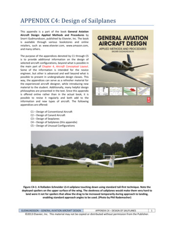
Dynamic soaring is utilized by many species of seabirds, some which use it to travel great distances. However, nobird species rivals the Albatross, who regularly travel thousands of miles in a single trip, with minimal flapping ofthe wings, effectively gliding across oceans. Among humans, the method is used both among pilots of sailplanesand radio-controlled aircraft.Long distance flying in sailplanes simply involves taking advantage of the energy available in the atmosphere thatcan be used to maintain necessary altitude. The pilot will ride the lift as high as possible before proceeding to thenext source of rising air. As such, the typical cross-country sailplane flight consists of a climb, followed by adescent, followed by another climb, and so forth. It is possible to reach very high altitudes in the process. Altitudesexceeding 30000 ft is a common occurrence and certainly requires an oxygen bottle to be carried along. Thethcurrent altitude record in a sailplane is 50722 ft (15460 m), set on 29 of August, 2006 by the Americans Steve3Fossett (1944-2007) and Einar Enevoldson, in a modified Glaser-Dirks DG-505 Open Class sailplane . The currentndlong range record stands at about 1214 nm (2248 km), set by Klaus Ohlman on 2 of December, 2003, on a4Schempp-Hirth Nimbus Open Class sailplane .Sailplane AirfoilsThe modern sailplane uses sophisticated NLFairfoils, capable of sustaining laminar boundarylayer up to 75% of the chord on the upper surfaceand 95% on the lower one. It is to be expectedthat such airfoils would yield lift and dragcharacteristics that are quite different fromairfoils typically selected for powered airplanes.This leads to a new paradigm in sailplane design:Standard drag models are usually abandoned, asare conventional performance analysis methodsthat are associated with them. Instead,performance must be based on drag modelingthat accurately accounts for the size of the dragbucket.Many sailplanes feature “cruise” flaps, which ismeans to raise the normal flaps a few degreesTrailing Edge Up (TEU) above neutral deflection.This shifts the drag polar toward a lower CL and,therefore, the L/D curve as well. Therefore, themaximum Lift-to-Drag (LDmax) is achievable at ahigher airspeed, which is very beneficial in longdistance competition. A typical drag polar and L/Dgraph for a modern sailplane airfoil is shown inFigure C4-4. The unconventional shape of the L/Dcurve is evident.Figure C4-4: Lift and drag characteristics of a typical modernsailplane airfoil. The graph is based on experimental datafrom Reference 5.Sailplanes generally operate at Reynolds Numbers that places their airfoils close to where the boundary layer issensitive to transition from laminar to turbulent (see Figure C4-5); the transition region. It is bounded on the lowerend by an expedited transition in high-turbulence environment (e.g. as encountered in wind tunnels) and theupper by what is possible in smooth atmosphere. To take advantage of the low drag associated with laminarboundary layer and to delay the transition of the boundary layer requires very smooth surfaces.GUDMUNDSSON – GENERAL AVIATION AIRCRAFT DESIGNAPPENDIX C4 – DESIGN OF SAILPLANES 2013 Elsevier, Inc. This material may not be copied or distributed without permission from the Publisher.4

Figure C4-5: Sailplanes operate in the transition region and must feature smooth surfaces to delay transitionfrom laminar to turbulent boundary layer. (Adapted from Reference 6)The Importance of the Drag BucketFigure C4-6 is an idealized representationintended to show the importance ofachieving NLF on a hypothetical sailplane.The shape of both the drag polar and L/Dcurve is classical for all NLF airfoils thatfeature a distinct two-wall drag bucket,including the double peak shape of the L/Dcurve. For instance, this characteristic ispresent in most NACA 65- and 66-seriesairfoils. The figure shows the impact this hason the glide performance of a hypotheticalsailplane. Reducing the CDmin by 30 dragcounts (e.g. from 0.013 to 0.010) increasesthe maximum L/D ratio by 4.2 units andshifts its location to a much lower CL. LowerCL means the LDmax will be realized at higherairspeed; something very beneficial to asailplane (and would be to a powered cruiseras well). Admittedly 30 drag counts are onthe high end of drag reduction and often thedrag characteristics of the airplane as awhole mask the presence of the drag bucket,so a distinct double-peak LD curves is notalways achieved for many applications.Instead, the laminar bucket shifts or widensthe range of CL, where “near” LDmaxperformance is found.Figure C4-6: Example of the benefit of achieving NLF on ahypothetical sailplane.GUDMUNDSSON – GENERAL AVIATION AIRCRAFT DESIGNAPPENDIX C4 – DESIGN OF SAILPLANES 2013 Elsevier, Inc. This material may not be copied or distributed without permission from the Publisher.5

As an example of the flexibility this yields, consider two sailplanes, A and B, which are identical except A does notdevelop a laminar drag bucket, while B does. Assume a wing loading of 10 lbf/ft² and that they are subject to theglide characteristics presented in Figure C4-6 (i.e. turbulent and laminar drag). Now consider a T-O scenario inwhich the sailplanes are towed to an altitude of 1500 ft AGL on a calm, sunny day and set out to reach a thermalsome 4 nm away. Naturally, if the thermal is absent, the pilots must return to base, which begs the question; isthere enough altitude remaining for the return flight? Using the performance methods of Chapter 21, Performance- Descent and noting that maintaining the airspeed for LDmax minimizes altitude loss, it is easy to show thatSailplane A achieves its LDmax at 58 KTAS, while B achieves it at 77 KTAS. It will take Sailplane A about 4m09s tocover a distance of 4 nm, while B covers it in 3m07s. Sailplane A loses 719 ft of altitude in the process and, uponreturn will be about 62 ft above the ground, requiring perfect piloting for the entire duration of the flight. SailplaneB loses 640 ft of altitude and will have some 220 ft upon return. Naturally, things are more complicated than this,although, in effect, this makes the point that a capable sailplane needs more than just a high LDmax; it should alsoachieve it at the lowest CL possible.Figure C4-7: Glide range for two identical sailplanes. Sailplane A does not develop NLF, but B does.Classes of SailplanesThe mission definition of sailplanes depends on factors such as how and where it is going to be used. Is it intendedfor training, competition, aerobatics, and so on? And what is the nature of updrafts it should be designed tooperate in; in other words, is it thermals or mountain waves? Sailplane design is also contingent upon the “class” itis slated for, as defined by the Fédération Aéronautique Internationale (FAI - The World Air Sports Federation) andlisted in Table C4-1:Table C4-1: Classes of Competition Sailplanes per FAI Definition.Class NameDescriptionOpen ClassNo restrictions. Max mass is 850 kg (1875 lbf)Standard Class18 meter ClassMax wingspan 15 m (49.2 ft), no camber changing devices, max mass is 525 kg (1159 lbf)Max wingspan 15 m (49.2 ft), camber changing devices permitted, max mass is 525 kg(1159 lbf)Max wingspan 18 m (59.1 ft), max mass is 600 kg (1325 lbf)20 meter Two-Seater ClassMax wingspan 20 m (65.6 ft), max mass is 750 kg (1656 lbf)World classLimited class for a single type of sailplane – the PW-5Club ClassFor older and smaller gliders. Handicap system is used to level the playing field.15 meter ClassGUDMUNDSSON – GENERAL AVIATION AIRCRAFT DESIGNAPPENDIX C4 – DESIGN OF SAILPLANES 2013 Elsevier, Inc. This material may not be copied or distributed without permission from the Publisher.6

C4.1.2 Sailplane Glide PerformanceSince the standard operation of sailplanes excludes the use of power (self-launching sailplanes glide with enginepower off), their flight is far more influenced by the presence of rising and sinking air, as well as head- andtailwinds. A deep understanding of glide performance is imperative for sailplane pilots, in particular whenattempting to maximize range. This section focuses on a few important elements of glide performance. It is largely72689based on references such as Reichmann , Welch and Irving , Thomas , Stewart , and Scull . In order to help explainthe fundamentals of glide performance, the properties of Sailplane A, discussed above, will be utilized in thefollowing discussion. To keep things manageable, a simplified quadratic drag model is used, given by CD 0.010 0.01498 CL². Also, time is represented using a format in which 6.25 minutes would be written as 6m15s.Glide Range and Glide EnduranceThe glide range is the horizontal distance a gliding aircraft covers between two given altitudes. The maximumrange in still air is obtained by maintaining the airspeed for minimum glide angle (or best angle of descent),denoted by VBG. The glide endurance is the time that takes a gliding aircraft to descent between two givenaltitudes. The maximum endurance in still air is obtained maintaining the airspeed for minimum rate of descent,denoted by VBA. This is shown schematically in Figure C4-8.Figure C4-8: A simple schematic showing the impact of any particular airspeed on glide range and time aloft ofSailplane A, from an altitude of 1000 ft, assuming still air. In still air, VBG always yields the longest range and VBAthe longest time aloft. Values are obtained using a flight polar like the one in Figure C4-9.Basic Mathematical Relations for Glide PerformanceThe following expressions are derived in Chapter 21, Performance – Descent and are repeated here forconvenience. All assume pure unpowered glide in still air and the simplified drag model.Angle of descent:tan θ Rate of descent:VV Rate of descent:VV Sink rate while banking at φ :VV D1D L L/D W(21-8)DVV W (CL CD )2(3LρC C2D)(21-10)CW 3D2S CL2Wρ S2WC2W 32 D 3232ρ (C L cos φ) CD S C L cos φ ρ S(GUDMUNDSSON – GENERAL AVIATION AIRCRAFT DESIGN)(21-12)(21-13)APPENDIX C4 – DESIGN OF SAILPLANES 2013 Elsevier, Inc. This material may not be copied or distributed without permission from the Publisher.7

2 cos θ WρC L SEquilibrium glide speedV Airspeed of Minimum Sink Rate:V BA Minimum Angle-of-Descent:tan θmin Best glide speed (still air):VBG VLD max Glide range: C L Rglide h h L D CDWhere:(21-11)2 W k ρ S 3 C D min(21-14)1 4 k CD minLDmaxCD Drag coefficientCDmin Minimum drag coefficientCL Lift coefficientD Dragh Altitudek Lift-induced drag constantL LiftLDmax Maximum lift-to-drag ratioRglide Glide rangeS Reference wing area2k Wρ C D min S (21-15)(21-16)(21-17)V AirspeedVBA Airspeed of minimum rate of descentVBG Airspeed of best glide (where LDmax occurs)VV Vertical airspeedW Weightφ Bank angleθ Glide angleθmin Minimum glide angleρ Air densityThe Basic Speed Polar – Optimum Glide in Still AirSailplane glide performance is determined using thespeed polar (also called a flight polar); a diagram thatshows the Rate-of-Descent (ROD) as a function ofairspeed (for instance, see Section 21.3.2, General Rateof Descent). This is obtained by plotting the product –60 D V/W versus airspeed.Consider the basic speed polar of Figure C4-9, whichshows the glide characteristics in still air and in theabsence of lift or sink. Note that if the sailplane losesaltitude, the value of the ROD is negative. A positiveROD means the sailplane is gaining altitude (climbing).Three important parameters are indicated; the stallingspeed, VS, the airspeeds of minimum ROD, VBA, andminimum glide angle, VBG. It can be seen that SailplaneA achieves a minimum ROD of 131 fpm at airspeed of 46KCAS (VBA) and LDmax of 40.9 is achieved at 60 KCAS(VBG). The ROD at VBG is 149 fpm. Maintaining VBA willyield the longest time aloft (endurance), and VBG yieldsthe greatest distance flown (range). These are optimumvalues in no-wind, no-thermal conditions only.GUDMUNDSSON – GENERAL AVIATION AIRCRAFT DESIGNFigure C4-9: Basic speed polar for Sailplane A at S-L.APPENDIX C4 – DESIGN OF SAILPLANES 2013 Elsevier, Inc. This material may not be copied or distributed without permission from the Publisher.8

In the world of sailplane piloting, the stalling speed (VS)is always indicated where the speed polar is terminatedon the left hand side (see Figure C4-9). Note that thestalling speed shown leads to an unrealistically highCLmax, a fact we will conveniently ignore, as said sailplaneis purely intended for explaining concepts.It is important to keep the basic speed polar in mindwhen considering sailplanes subject to lift or sink andhead- or tailwind.The Speed Polar with Variable Wing LoadingThe speed polar for the sailplane is often prepared withone or two specific and frequently used weights inmind. If the sailplane is loaded to higher weight, forinstance, due to the addition of a second occupant orwater ballast) the speed polar will be shifted to a higherairspeed when compared to the polar at a lighter weight(see Figure C4-10). The general rule-of-thumb is thatthere is no change in the LDmax, only in the airspeed atwhich it occurs. On the other hand, and as is to beexpected, the magnitude of RODmin increases, as doesthe airspeed at which it occurs. The figure shows this isakin to sliding the polar along the sloped line, althoughit also “expands” as shown.Figure C4-10: Basic speed polar for Sailplane A at S-L,while subject to 30% increase in weight.In the case of Sailplane A, there is no change in the magnitude of the LDmax, but its airspeed increases from 60 to69 KCAS with a 30% increase in weight. The magnitude of RODmin increases from 131 to 149 fpm and its airspeedfrom 46 to 52 KCAS.Optimum Glide in Sinking AirIf the sailplane enters a column of air sinking at some average rate, say 200 fpm (about 2 knots), this is akin toshifting the speed polar downward as shown in the left graph of Figure C4-11. It can be seen that this does notaffect VBA. However, VBG is shifted to a higher airspeed, here, from 60 to 77 KCAS. As stated before, in the absenceof lift or sink, the normal ROD at these two airspeeds is 131 (at VBA) and 148 fpm (at VBG), respectively. Theeffective LDmax (defined here as horizontal speed divided by the vertical speed) is reduced from 40.9 to 18.8. Notethat it is not important whether the polar is shifted downward or the origin is shifted upward, as shown in the rightgraph of Figure C4-11. The right graph, thus, presents a clever method to determine the best airspeed-to-fly usinga polar made for standard conditions only. This is discussed in more detail later.To help understand why it is beneficial to increase the airspeed, assume the sailplane glides right through thecenter of a column of uniformly sinking air, whose diameter is 1 nm, and average rate is 200 fpm. At 60 KCAS, itwill take the sailplane one minute flat to fly through the column, during which it is descends at 131 200 331fpm. In other words, it loses 331 ft of altitude in the process. At 77 KCAS, the sailplane descends at 148 200 348fpm and it will take 47 seconds to cruise through the column, during which it loses (47/60) x 348 273 ft.Therefore, less altitude is lost by flying at the higher airspeed. While the difference (58 ft) may seem trivial, it is ofcrucial importance to the precision piloting required to fly long distances competitively.Figure C4-12 shows how the downdraft affects the glide from a different perspective; presenting it as L/D versusairspeed. The peak L/D is reduced and shifted to a higher airspeed.GUDMUNDSSON – GENERAL AVIATION AIRCRAFT DESIGNAPPENDIX C4 – DESIGN OF SAILPLANES 2013 Elsevier, Inc. This material may not be copied or distributed without permission from the Publisher.9

Optimum Glide in Rising AirIf the sailplane enters a column of air rising at some average rate, say 200 fpm, this corresponds to shifting thespeed polar upward by that amount, as shown in Figure C4-13. Again, this has no effect on VBA, which now isanalogous to VY (best Rate-of-Climb airspeed) for powered aircraft. Similarly, VBG becomes the best-angle-of-climbairspeed (denoted by VX for powered aircraft) and it should maintained in a straight and level flight inside athermal to achieve the steepest climb angle (although flying in thermals usually requires circling flight, so this isnot as simple as that). Note that shifting the polar downward or the origin upward yields the same answer (seeFigure C4-11).Figure C4-11: The speed polar for Sailplane A, assuming it enters a column of air sinking at 200 fpm ( 2 knots or1 m/s). Both graphs display the same information. By shifting the origin of the vertical axis in the right graph upby 200 fpm, exactly the same answer is obtained as in the left graph.Optimum Glide in Headwind or TailwindConsider Sailplane A gliding in a 10 knot headwind (ortailwind) while the pilot maintains a constantcalibrated airspeed of 60 KCAS (i.e. by keeping theneedle of the airspeed indicator pointing at 60 KCAS).With respect to the ground, the aforementioned glidespeeds will occur 10 knots slower (or faster). This way,the normal best angle glide speed of 60 KCAS (VBG) willactually correspond to 50 (or 70) KGS (Knots GroundSpeed). If the pilot maintains 60 KCAS, the glide rangeof the sailplane (descending at 148 fpm) will varygreatly. The same holds for the glide angle, θ, withrespect to the ground, which can be determined asfollows:Figure C4-12: Standard and “effective” L/D curves forSailplane A at S-L. The sink rate is 200 fpm.GUDMUNDSSON – GENERAL AVIATION AIRCRAFT DESIGNAPPENDIX C4 – DESIGN OF SAILPLANES 2013 Elsevier, Inc. This material may not be copied or distributed without permission from the Publisher.10

In a 10 knot tailwind:In no-wind conditions:In a 10 knot headwind:θ tan 1 [(148 / 60 ) (70 1.688)] 1.20 θ 0.20 [(148 / 60) (60 1.688)] 1.40 [(148 / 60) (50 1.688)] 1.67 θ 0.27 θ tan 1θ tan 1Where θ represents the difference between the still air and windy glide-angle condition. This is shownschematically in Figure C4-14. If the sailplane begins its glide 1000 ft above the ground, it will touch down in1000/148 6m45s in all three cases, however, the range in headwind will be approximately (50 nm/60 min) x (6.75min) 5.63 nm, 6.76 nm in still air, and 7.88 nm in tailwind.Figure C4-13: The speed polar for Sailplane A, assuming it enters a lift of 200 fpm ( 2 knots or 1 m/s). Bothgraphs display the same information. By shifting the origin of the vertical axis in the right graph down by 200fpm, exactly the same answer is obtained as that in the left graph.Figure C4-14: A simple schematic showing the impact of head- or tailwind on the glide range assuming the pilotmaintains the same indicated (or calibrated) airspeed in all three cases.This begs the question: In headwind, is there an airspeed other than 60 KCAS that yields range greater than 5.63nm? To answer this question, assume that this time Sailplane A is being flown in a 10 knot headwind at 63 KCAS.GUDMUNDSSON – GENERAL AVIATION AIRCRAFT DESIGNAPPENDIX C4 – DESIGN OF SAILPLANES 2013 Elsevier, Inc. This material may not be copied or distributed without permission from the Publisher.11

The ROD at this airspeed is 156 fpm. The ground speed will be 53 KGS and the glide will last for 1000/156 6m24s(approximately 6.40 min). In that time, it will cover (53 nm/60 min) x (6.40 min) 5.65 nm, which is greater than5.63 nm at 60 KCAS. This shows that increasing the airspeed (up to a certain point) in headwind, yields greaterrange. The inverse is true for tailwind.It should be clear that a sailplane gliding in headwind equal to its forward speed in magnitude will not make anyheadway with respect to the ground. Rather it would descend vertically – its glide angle would be 90 . Horizontaldistance can only be achieved by a forward glide speed faster than the headwind. The airspeed that yields thegreatest range can be determined by shifting the origin of the speed polar horizontally by a distance that equalsthe wind speed, and then draw a tangent to the speed polar. Like the previous discussion demonstrates, inheadwind, the origin of the coordinate system is shifted sideways to the right, while for tailwind it is shifted to theleft, as shown in Figure C4-15.Figure C4-15: The speed polar for Sailplane A, for a glide in a 10 knot tail- and headwind. By shifting the origin ofthe horizontal axis to the left or right by 10 knots, an ideal airspeed for glide is obtained.Speed-to-FlyThe preceding discussion shows that a speed polar for no wind, no thermal conditions can be used with ease todetermine the proper airspeed to fly in any non-standard conditions in order to maximize the range of thesailplane. The particular airspeed obtained this way is referred to as Speed-to-Fly by sailplane pilots. It isdetermined by shifting the origin around as shown in Figure C4-17. For headwind, the origin is shifted to the right.For headwind and sink, it is shifted to the right and up, and so on.Average Cross-Country SpeedPhysics

maximum Lift-to-Drag (LD max) is achievable at a higher airspeed, which is very beneficial in long distance competition. A typical drag polar and L/D graph for a modern sailplane airfoil is shown in Figure C4-4. The unconventional shape of the L/D curve is evident. Figure C4-4: Lift and dr