Transcription
Introduction to the Economics and Mathematics of Financial Markets
This page intentionally left blank
Introduction to the Economics and Mathematics of Financial MarketsJakša Cvitanić and Fernando ZapateroThe MIT PressCambridge, MassachusettsLondon, England
c 2004 Massachusetts Institute of Technology All rights reserved. No part of this book may be reproduced in any form by any electronic or mechanical means(including photocopying, recording, or information storage and retrieval) without permission in writing from thepublisher.This book was set in 10/13 Times Roman by ICC and was printed and bound in the United States of America.Library of Congress Cataloging-in-Publication DataCvitanić, JakšaIntroduction to the economics and mathematics of financial markets / Jakša Cvitanić andFernando Zapatero.p.cm.Includes bibliographical references and index.ISBN 0-262-03320-8ISBN 0-262-53265-4 (International Student Edition)1. Finance—Mathematical models—Textbooks. I. Zapatero, Fernando. II. Title.HG106.C86 2004332.632 01 515—dc222003064872
To Vesela, Lucia, ToniandMaitica, Nicolás, Sebastián
This page intentionally left blank
ContentsPrefaceI11.11.21.31.41.51.622.1THE SETTING: MARKETS, MODELS, INTEREST RATES,UTILITY MAXIMIZATION, RISKxvii1Financial MarketsBonds1.1.1 Types of Bonds1.1.2 Reasons for Trading Bonds1.1.3 Risk of Trading BondsStocks1.2.1 How Are Stocks Different from Bonds?1.2.2 Going Long or ShortDerivatives1.3.1 Futures and Forwards1.3.2 Marking to Market1.3.3 Reasons for Trading Futures1.3.4 Options1.3.5 Calls and Puts1.3.6 Option Prices1.3.7 Reasons for Trading Options1.3.8 Swaps1.3.9 Mortgage-Backed Securities; Callable BondsOrganization of Financial Markets1.4.1 Exchanges1.4.2 Market IndexesMargins1.5.1 Trades That Involve Margin RequirementsTransaction CostsSummaryProblemsFurther 629Interest RatesComputation of Interest Rates2.1.1 Simple versus Compound Interest; Annualized Rates2.1.2 Continuous Interest31313234
viii2.22.333.13.23.33.43.5ContentsPresent Value2.2.1 Present and Future Values of Cash Flows2.2.2 Bond Yield2.2.3 Price-Yield CurvesTerm Structure of Interest Rates and Forward Rates2.3.1 Yield Curve2.3.2 Calculating Spot Rates; Rates Arbitrage2.3.3 Forward Rates2.3.4 Term-Structure TheoriesSummaryProblemsFurther Readings353639394141434547484951Models of Securities Prices in Financial MarketsSingle-Period Models3.1.1 Asset Dynamics3.1.2 Portfolio and Wealth Processes3.1.3 Arrow-Debreu SecuritiesMultiperiod Models3.2.1 General Model Specifications3.2.2 Cox-Ross-Rubinstein Binomial ModelContinuous-Time Models3.3.1 Simple Facts about the Merton-Black-Scholes Model3.3.2 Brownian Motion Process3.3.3 Diffusion Processes, Stochastic Integrals3.3.4 Technical Properties of Stochastic Integrals 3.3.5 Itô’s Rule3.3.6 Merton-Black-Scholes Model3.3.7 Wealth Process and Portfolio ProcessModeling Interest Rates3.4.1 Discrete-Time Models3.4.2 Continuous-Time ModelsNominal Rates and Real Rates3.5.1 Discrete-Time Models3.5.2 Continuous-Time Models53545455575858606262636667697478797980818183
Contents3.63.744.14.24.34.44.54.6ixArbitrage and Market Completeness3.6.1 Notion of Arbitrage3.6.2 Arbitrage in Discrete-Time Models3.6.3 Arbitrage in Continuous-Time Models3.6.4 Notion of Complete Markets3.6.5 Complete Markets in Discrete-Time Models3.6.6 Complete Markets in Continuous-Time Models Appendix3.7.1 More Details for the Proof of Itô’s Rule3.7.2 Multidimensional Itô’s RuleSummaryProblemsFurther Readings838485868788929494979798101Optimal Consumption / Portfolio StrategiesPreference Relations and Utility Functions4.1.1 Consumption4.1.2 Preferences4.1.3 Concept of Utility Functions4.1.4 Marginal Utility, Risk Aversion, and Certainty Equivalent4.1.5 Utility Functions in Multiperiod Discrete-Time Models4.1.6 Utility Functions in Continuous-Time ModelsDiscrete-Time Utility Maximization4.2.1 Single Period4.2.2 Multiperiod Utility Maximization: Dynamic Programming4.2.3 Optimal Portfolios in the Merton-Black-Scholes Model4.2.4 Utility from ConsumptionUtility Maximization in Continuous Time4.3.1 Hamilton-Jacobi-Bellman PDEDuality/Martingale Approach to Utility Maximization4.4.1 Martingale Approach in Single-Period Binomial Model4.4.2 Martingale Approach in Multiperiod Binomial Model4.4.3 Duality/Martingale Approach in Continuous Time Transaction CostsIncomplete and Asymmetric Information4.6.1 Single 2128128130133138139139
xContents4.6.2 Incomplete Information in Continuous Time 4.6.3 Power Utility and Normally Distributed Drift Appendix: Proof of Dynamic Programming PrincipleSummaryProblemsFurther Readings140142145146147150RiskRisk versus Return: Mean-Variance Analysis5.1.1 Mean and Variance of a Portfolio5.1.2 Mean-Variance Efficient Frontier5.1.3 Computing the Optimal Mean-Variance Portfolio5.1.4 Computing the Optimal Mutual Fund5.1.5 Mean-Variance Optimization in Continuous Time VaR: Value at Risk5.2.1 Definition of VaR5.2.2 Computing VaR5.2.3 VaR of a Portfolio of Assets5.2.4 Alternatives to VaR5.2.5 The Story of Long-Term Capital ManagementSummaryProblemsFurther 172175IIPRICING AND HEDGING OF DERIVATIVE SECURITIES17766.16.2Arbitrage and Risk-Neutral PricingArbitrage Relationships for Call and Put Options; Put-Call ParityArbitrage Pricing of Forwards and Futures6.2.1 Forward Prices6.2.2 Futures Prices6.2.3 Futures on CommoditiesRisk-Neutral Pricing6.3.1 Martingale Measures; Cox-Ross-Rubinstein (CRR) Model6.3.2 State Prices in Single-Period Models6.3.3 No Arbitrage and Risk-Neutral 5.26.3
Contents6.477.17.27.37.47.5xi6.3.4 Pricing by No Arbitrage6.3.5 Pricing by Risk-Neutral Expected Values6.3.6 Martingale Measure for the Merton-Black-Scholes Model6.3.7 Computing Expectations by the Feynman-Kac PDE6.3.8 Risk-Neutral Pricing in Continuous Time6.3.9 Futures and Forwards Revisited Appendix6.4.1 No Arbitrage Implies Existence of a Risk-Neutral Probability 6.4.2 Completeness and Unique EMM 6.4.3 Another Proof of Theorem 6.4 6.4.4 Proof of Bayes’ Rule SummaryProblemsFurther Option PricingOption Pricing in the Binomial Model7.1.1 Backward Induction and Expectation Formula7.1.2 Black-Scholes Formula as a Limit of the BinomialModel FormulaOption Pricing in the Merton-Black-Scholes Model7.2.1 Black-Scholes Formula as Expected Value7.2.2 Black-Scholes Equation7.2.3 Black-Scholes Formula for the Call Option7.2.4 Implied VolatilityPricing American Options7.3.1 Stopping Times and American Options7.3.2 Binomial Trees and American Options7.3.3 PDEs and American Options Options on Dividend-Paying Securities7.4.1 Binomial Model7.4.2 Merton-Black-Scholes ModelOther Types of Options7.5.1 Currency Options7.5.2 Futures Options7.5.3 Exotic 36238240240242243
xii7.67.77.87.988.18.28.38.499.1ContentsPricing in the Presence of Several Random Variables7.6.1 Options on Two Risky Assets7.6.2 Quantos7.6.3 Stochastic Volatility with Complete Markets7.6.4 Stochastic Volatility with Incomplete Markets; Market Priceof Risk 7.6.5 Utility Pricing in Incomplete Markets Merton’s Jump-Diffusion Model Estimation of Variance and ARCH/GARCH ModelsAppendix: Derivation of the Black-Scholes FormulaSummaryProblemsFurther Readings247248252255Fixed-Income Market Models and DerivativesDiscrete-Time Interest-Rate Modeling8.1.1 Binomial Tree for the Interest Rate8.1.2 Black-Derman-Toy Model8.1.3 Ho-Lee ModelInterest-Rate Models in Continuous Time8.2.1 One-Factor Short-Rate Models8.2.2 Bond Pricing in Affine Models8.2.3 HJM Forward-Rate Models8.2.4 Change of Numeraire 8.2.5 Option Pricing with Random Interest Rate 8.2.6 BGM Market Model Swaps, Caps, and Floors8.3.1 Interest-Rate Swaps and Swaptions8.3.2 Caplets, Caps, and FloorsCredit/Default RiskSummaryProblemsFurther 305306308309312HedgingHedging with Futures9.1.1 Perfect Hedge313313313256257260262265267268273
Contents9.29.39.49.59.1.2 Cross-Hedging; Basis Risk9.1.3 Rolling the Hedge Forward9.1.4 Quantity UncertaintyPortfolios of Options as Trading Strategies9.2.1 Covered Calls and Protective Puts9.2.2 Bull Spreads and Bear Spreads9.2.3 Butterfly Spreads9.2.4 Straddles and StranglesHedging Options Positions; Delta Hedging9.3.1 Delta Hedging in Discrete-Time Models9.3.2 Delta-Neutral Strategies9.3.3 Deltas of Calls and Puts9.3.4 Example: Hedging a Call Option9.3.5 Other Greeks9.3.6 Stochastic Volatility and Interest Rate9.3.7 Formulas for Greeks9.3.8 Portfolio InsurancePerfect Hedging in a Multivariable Continuous-Time ModelHedging in Incomplete MarketsSummaryProblemsFurther Readings10 Bond Hedging10.1 Duration10.1.1 Definition and Interpretation10.1.2 Duration and Change in Yield10.1.3 Duration of a Portfolio of Bonds10.2 Immunization10.2.1 Matching Durations10.2.2 Duration and Immunization in Continuous Time10.3 ConvexitySummaryProblemsFurther 50351352352353
xivContents11 Numerical Methods11.1 Binomial Tree Methods11.1.1 Computations in the Cox-Ross-Rubinstein Model11.1.2 Computing Option Sensitivities11.1.3 Extensions of the Tree Method11.2 Monte Carlo Simulation11.2.1 Monte Carlo Basics11.2.2 Generating Random Numbers11.2.3 Variance Reduction Techniques11.2.4 Simulation in a Continuous-Time Multivariable Model11.2.5 Computation of Hedging Portfolios by Finite Differences11.2.6 Retrieval of Volatility Method for Hedging andUtility Maximization 11.3 Numerical Solutions of PDEs; Finite-Difference Methods11.3.1 Implicit Finite-Difference Method11.3.2 Explicit Finite-Difference MethodSummaryProblemsFurther ILIBRIUM MODELS12 Equilibrium Fundamentals12.1 Concept of Equilibrium12.1.1 Definition and Single-Period Case12.1.2 A Two-Period Example12.1.3 Continuous-Time Equilibrium12.2 Single-Agent and Multiagent Equilibrium12.2.1 Representative Agent12.2.2 Single-Period Aggregation12.3 Pure Exchange Equilibrium12.3.1 Basic Idea and Single-Period Case12.3.2 Multiperiod Discrete-Time Model12.3.3 Continuous-Time Pure Exchange Equilibrium12.4 Existence of Equilibrium12.4.1 Equilibrium Existence in Discrete 91392394395398399
Contentsxv12.4.2 Equilibrium Existence in Continuous Time12.4.3 Determining Market Parameters in EquilibriumSummaryProblemsFurther Readings40040340640640713 CAPM13.1 Basic CAPM13.1.1 CAPM Equilibrium Argument13.1.2 Capital Market Line13.1.3 CAPM formula13.2 Economic Interpretations13.2.1 Securities Market Line13.2.2 Systematic and Nonsystematic Risk13.2.3 Asset Pricing Implications: Performance Evaluation13.2.4 Pricing Formulas13.2.5 Empirical Tests13.3 Alternative Derivation of the CAPM 13.4 Continuous-Time, Intertemporal CAPM 13.5 Consumption CAPM SummaryProblemsFurther 445445Multifactor ModelsDiscrete-Time Multifactor ModelsArbitrage Pricing Theory (APT)Multifactor Models in Continuous Time 14.3.1 Model Parameters and Variables14.3.2 Value Function and Optimal Portfolio14.3.3 Separation Theorem14.3.4 Intertemporal Multifactor CAPMSummaryProblemsFurther Readings
xviContents15 Other Pure Exchange Equilibria15.1 Term-Structure Equilibria15.1.1 Equilibrium Term Structure in Discrete Time15.1.2 Equilibrium Term Structure in Continuous Time; CIR Model15.2 Informational Equilibria15.2.1 Discrete-Time Models with Incomplete Information15.2.2 Continuous-Time Models with Incomplete Information15.3 Equilibrium with Heterogeneous Agents15.3.1 Discrete-Time Equilibrium with Heterogeneous Agents15.3.2 Continuous-Time Equilibrium with Heterogeneous Agents15.4 International Equilibrium; Equilibrium with Two Prices15.4.1 Discrete-Time International Equilibrium15.4.2 Continuous-Time International EquilibriumSummaryProblemsFurther 46646716 Appendix: Probability Theory Essentials16.1 Discrete Random Variables16.1.1 Expectation and Variance16.2 Continuous Random Variables16.2.1 Expectation and Variance16.3 Several Random Variables16.3.1 Independence16.3.2 Correlation and Covariance16.4 Normal Random Variables16.5 Properties of Conditional Expectations16.6 Martingale Definition16.7 Random Walk and Brownian esIndex479487
PrefaceWhy We Wrote the BookThe subject of financial markets is fascinating to many people: to those who care aboutmoney and investments, to those who care about the well-being of modern society, to thosewho like gambling, to those who like applications of mathematics, and so on. We, theauthors of this book, care about many of these things (no, not the gambling), but whatwe care about most is teaching. The main reason for writing this book has been our beliefthat we can successfully teach the fundamentals of the economic and mathematical aspectsof financial markets to almost everyone (again, we are not sure about gamblers). Why arewe in this teaching business instead of following the path of many of our former students,the path of making money by pursuing a career in the financial industry? Well, they don’thave the pleasure of writing a book for the enthusiastic reader like yourself!PrerequisitesThis text is written in such a way that it can be used at different levels and for different groupsof undergraduate and graduate students. After the first, introductory chapter, each chapterstarts with sections on the single-period model, goes to multiperiod models, and finisheswith continuous-time models. The single-period and multiperiod models require only basiccalculus and an elementary introductory probability/statistics course. Those sections canbe taught to third- and fourth-year undergraduate students in economics, business, andsimilar fields. They could be taught to mathematics and engineering students at an evenearlier stage. In order to be able to read continuous-time sections, it is helpful to have beenexposed to an advanced undergraduate course in probability. Some material needed fromsuch a probability course is briefly reviewed in chapter 16.Who Is It For?The book can also serve as an introductory text for graduate students in finance, financial economics, financial engineering, and mathematical finance. Some material from continuoustime sections is, indeed, usually considered to be graduate material. We try to explain muchof that material in an intuitive way, while providing some of the proofs in appendixes tothe chapters. The book is not meant to compete with numerous excellent graduate-levelbooks in financial mathematics and financial economics, which are typically written in amathematically more formal way, using a theorem-proof type of structure. Some of thosemore advanced books are mentioned in the references, and they present a natural next stepin getting to know the subject on a more theoretical and advanced level.
xviiiPrefaceStructure of the BookWe have divided the book into three parts. Part I goes over the basic securities, organizationof financial markets, the concept of interest rates, the main mathematical models, andways to measure in a quantitative way the risk and the reward of trading in the market.Part II deals with option pricing and hedging, and similar material is present in virtuallyevery recent book on financial markets. We choose to emphasize the so-called martingale,probabilistic approach consistently throughout the book, as opposed to the differentialequations approach or other existing approaches. For example, the one proof of the BlackScholes formula that we provide is done calculating the corresponding expected value.Part III is devoted to one of the favorite subjects of financial economics, the equilibriumapproach to asset pricing. This part is often omitted from books in the field of financialmathematics, having fewer direct applications to option pricing and hedging. However, it isthis theory that gives a qualitative insight into the behavior of market participants and howthe prices are formed in the market.What Can a Course Cover?We have used parts of the material from the book for teaching various courses at the University of Southern California: undergraduate courses in economics and business, a masterslevel course in mathematical finance, and option and investment courses for MBA students.For example, an undergraduate course for economics/business students that emphasizesoption pricing could cover the following (in this order):The first three chapters without continuous-time sections; chapter 10 on bond hedgingcould also be done immediately after chapter 2 on interest rates The first two chapters of part II on no-arbitrage pricing and option pricing, without mostof the continuous-time sections, but including basic Black-Scholes theory Chapters on hedging in part II, with or without continuous-time sectionsThe mean-variance section in chapter 5 on risk; chapter 13 on CAPM could also be doneimmediately after that section If time remains, or if this is an undergraduate economics course that emphasizesequilibrium/asset pricing as opposed to option pricing, or if this is a two-semester course,one could also cover discrete-time sections in chapter 4 on utility. discrete-time sections in part III on equilibrium models.
PrefacexixCourses aimed at more mathematically oriented students could go very quickly throughthe discrete-time sections, and instead spend more time on continuous-time sections. Aone-semester course would likely have to make a choice: to focus on no-arbitrage optionpricing methods in part II or to focus on equilibrium models in part III.Web Page for This Book, Excel FilesThe web page http://math.usc.edu/ cvitanic/book.html will be regularly updated withmaterial related to the book, such as corrections of typos. It also contains Microsoft Excelfiles, with names like ch1.xls. That particular file has all the figures from chapter 1, alongwith all the computations needed to produce them. We use Excel because we want the readerto be able to reproduce and modify all the figures in the book. A slight disadvantage of thischoice is that our figures sometimes look less professional than if they had been done by aspecialized drawing software. We use only basic features of Excel, except for Monte Carlosimulation for which we use the Visual Basic programming language, incorporated in Excel.The readers are expected to learn the basic features of Excel on their own, if they are notalready familiar with them. At a few places in the book we give “Excel Tips” that point outthe trickier commands that have been used for creating a figure. Other, more mathematicallyoriented software may be more efficient for longer computations such as Monte Carlo, andwe leave the choice of the software to be used with some of the homework problems to theinstructor or the reader. In particular, we do not use any optimization software or differentialequations software, even though the instructor could think of projects using those.NotationAsterisk Sections and problems designated by an asterisk are more sophisticated in mathematical terms, require extensive use of computer software, or are otherwise somewhatunusual and outside of the main thread of the book. These sections and problems couldbe skipped, although we suggest that students do most of the problems that require use ofcomputers.Dagger End-of-chapter problems that are solved in the student’s manual are preceded bya dagger.Greek Letters We use many letters from the Greek alphabet, sometimes both lowercaseand uppercase, and we list them here with appropriate pronunciation: α (alpha), β (beta),γ , (gamma), δ, (delta), ε (epsilon), ζ (zeta), η (eta), θ (theta), λ (lambda), μ (mu),ξ (xi), π, (pi), ω, (omega), ρ (rho), σ, (sigma), τ (tau), ϕ, (phi).
xxPrefaceAcknowledgmentsFirst and foremost, we are immensely grateful to our families for the support they providedus while working on the book. We have received great help and support from the staff of ourpublisher, MIT Press, and, in particular, we have enjoyed working with Elizabeth Murry,who helped us go through the writing and production process in a smooth and efficientmanner. J. C.’s research and the writing of this book have been partially supported byNational Science Foundation grant DMS-00-99549. Some of the continuous-time sectionsin parts I and II originated from the lecture notes prepared in summer 2000 while J. C. wasvisiting the University of the Witwatersrand in Johannesburg, and he is very thankful tohis host, David Rod Taylor, the director of the Mathematical Finance Programme at Wits.Numerous colleagues have made useful comments and suggestions, including KrzysztofBurdzy, Paul Dufresne, Neil Gretzky, Assad Jalali, Dmitry Kramkov, Ali Lazrak, LionelMartellini, Adam Ostaszewski, Kaushik Ronnie Sircar, Costis Skiadas, Halil Mete Soner,Adam Speight, David Rod Taylor, and Mihail Zervos. In particular, D. Kramkov providedus with proofs in the appendix of chapter 6. Some material on continuous-time utilitymaximization with incomplete information is taken from a joint work with A. Lazrak andL. Martellini, and on continuous-time mean-variance optimization from a joint work withA. Lazrak. Moreover, the following students provided their comments and pointed outerrors in the working manuscript: Paula Guedes, Frank Denis Hiebsch, and Chulhee Lee.Of course, we are solely responsible for any remaining errors.A Prevailing Theme: Pricing by Expected ValuesBefore we start with the book’s material, we would like to give a quick illustration here inthe preface of a connection between a price of a security and the optimal trading strategy ofan investor investing in that security. We present it in a simple model, but this connection ispresent in most market models, and, in fact, the resulting pricing formula is of the form thatwill follow us through all three parts of this book. We will repeat this type of argument laterin more detail, and we present it early here only to give the reader a general taste of whatthe book is about. The reader may want to skip the following derivation, and go directly toequation (0.3).Consider a security S with today’s price S(0), and at a future time 1 its price S(1) eitherhas value s u with probability p, or value s d with probability 1 p. There is also a risk-freesecurity that returns 1 r dollars at time 1 for every dollar invested today. We assume thats d (1 r )S(0) s u . Suppose an investor has initial capital x, and has to decide howmany shares δ of security S to hold, while depositing the rest of his wealth in the bank
Prefacexxiaccount with interest rate r . In other words, his wealth X (1) at time 1 isX (1) δS(1) [x δS(0)](1 r )The investor wants to maximize his expected utilityE[U (X (1))] pU (X u ) (1 p)U (X d )where U is a so-called utility function, while X u , X d is his final wealth in the case S(1) s u ,S(1) s d , respectively. Substituting for these values, taking the derivative with respect toδ and setting it equal to zero, we getpU (X u )[s u S(0)(1 r )] (1 p)U (X d )[s d S(0)(1 r )] 0The left-hand side can be written as E[U (X (1)){S(1) S(0)(1 r )}], which, when madeequal to zero, implies, with arbitrary wealth X replaced by optimal wealth X̂ , U ( X̂ (1)) S(1)(0.1)S(0) EE(U [X̂ (1)]) 1 rIf we denoteZ (1) : U (X̂ (1))E{U (X̂ (1))}we see that the today’s price of our security S is given by S(1)S(0) E Z (1)1 r(0.2)(0.3)We will see that prices of most securities (with some exceptions, like American options)in the models of this book are of this form: the today’s price S(0) is an expected value ofthe future price S(1), multiplied (“discounted”) by a certain random factor. Effectively, weget the today’s price as a weighted average of the discounted future price, but with weightsthat depend on the outcomes of the random variable Z (1). Moreover, in standard optionpricing models (having a so-called completeness property) we will not need to use utilityfunctions, since Z (1) will be independent of the investor’s utility. The random variable Z (1)is sometimes called change of measure, while the ratio Z (1)/(1 r ) is called state-pricedensity, stochastic discount factor, pricing kernel, or marginal rate of substitution,depending on the context and interpretation. There is another interpretation of this formula,using a new probability; hence the name “change of (probability) measure.” For example,if, as in our preceding example, Z (1) takes two possible values Z u (1) and Z d (1) with
xxiiPrefaceprobabilities p, 1 p, respectively, we can definep : p Z u (1),1 p (1 p)Z d (1)The values of Z (1) are such that p is a probability, and we interpret p and 1 p asmodified probabilities of the movements of asset S. Then, we can write equation (0.3) as S(1)(0.4)S(0) E 1 rwhere E denotes the expectation under the new probabilities, p , 1 p . Thus the pricetoday is the expected value of the discounted future value, where the expected value iscomputed under a special, so-called risk-neutral probability, usually different from thereal-world probability.Final WordWe hope that we have aroused your interest about the subject of this book. If you turn out tobe a very careful reader, we would be thankful if you could inform us of any remainingtypos and errors that you find by sending an e-mail to our current e-mail addresses. Enjoythe book!Jakša Cvitanić and Fernando ZapateroE-mail addresses: cvitanic@math.usc.edu, zapatero@usc.edu
ITHE SETTING: MARKETS, MODELS, INTEREST RATES, UTILITYMAXIMIZATION, RISK
This page intentionally left blank
1Financial MarketsImagine that our dear reader (that’s you) was lucky enough to inherit one million dollarsfrom a distant relative. This is more money than you want to spend at once (we assume),and you want to invest some of it. Your newly hired expert financial adviser tells you that anattractive possibility is to invest part of your money in the financial market (and pay him ahefty fee for the advice, of course). Being suspicious by nature, you don’t completely trustyour adviser, and you want to learn about financial markets yourself. You do a smart thingand buy this book (!) for a much smaller fee that pays for the services of the publisher andthe authors (that’s us). You made a good deal because the learning objectives of the firstchapter areto describe the basic characteristics of and differences between the instruments traded infinancial markets. to provide an overview of the organization of financial markets.Our focus will be on the economic and financial use of financial instruments. There aremany possible classifications of these instruments. The first division differentiates betweensecurities and other financial contracts. A security is a document that confers upon its ownera financial claim. In contrast, a general financial contract links two parties nominally andnot through the ownership of a document. However, this distinction is more relevant forlegal than for economic reasons, and we will overlook it. We start with the broadest possibleeconomic classification: bonds, stocks, and derivatives. We describe the basic characteristicsof each type, its use from the point of view of an investor, and its organization in differentmarkets.Bonds belong to the family of fixed-income securities, because they pay fixed amountsof money to their owners. Other fixed-income instruments include regular savings accounts,money-market accounts, certificates of deposit, and others. Stocks are also referred to asequities. See figure 1.1 for a possible classification of financial instruments.The financial instruments discussed in this chapter are assets a potential investor wouldconsider as a part of his portfolio. This potential investor can be a person or an entity(a corporation, a pension fund, a country, . . .). In the economics and finance literature sucha person or entity may be called a trader, an agent, a financial investor, and similar terms.We will name this investor Taf.1.1BondsIn a very broad sense, a bond is a security (a document) that gives its owner the right to afixed, predetermined payment, at a future, predetermined date, called maturity. The amountof money that a bond will pay in the future is called nominal value, face value, par value,or principal.
4Chapter 1Securities and ContractsBasic SecuritiesFixed IncomeBondsBankaccountsDerivatives and ContractsEquities StocksOptionsCallsand putsSwapsFuturesand ForwardsExoticoptionsFigure 1.1A classification of financial instruments: financial securities and contracts.There are two sides to a bond contract: the party that promises to pay the nominal value,or the debtor, and the party that will get paid, or the creditor. We say that the debtor isa counterparty to the creditor in the bond contract, and vice versa. The debtor issues abond in exchange for an agreed-upon amount called the bond price paid by the creditor. Forexample, the creditor may have to pay 95.00 today for a bond that pays 100.00 a year fromtoday. The creditor can later sell the bond to another person who becomes the new creditor.The difference between the bond price the creditor pays to the debtor and the nominal valueis called interest. The interest as a percentage of the total value is called interest rate.Typically, but not always, a bond with longer maturity pays a higher interest rate. A bondis characterized by its interest and its maturity. In principle, bonds represent the paradigmof risk-free securities, in the sense that there is a guaranteed payoff at maturity, knownin advance. The lack of risk is the result o
1.3.6 Option Prices 15 1.3.7 Reasons for Trading Options 16 1.3.8 Swaps 17 1.3.9 Mortgage-Backed Securities; Callable Bonds 19 1.4 Organization of Financial Markets 20 1.4.1 Exchanges 20 1.4.2 Market Indexes 21 1.5 Margins 22 1.5.1 Trades That In