Transcription
THE TRAVELING SALESMAN PROBLEMbyCorinne BrucatoB.A., Sonoma State University, 2010M.S., University of Pittsburgh, 2013Submitted to the Graduate Faculty ofthe Department of Mathematics in partial fulfillmentof the requirements for the degree ofMaster of SciencesUniversity of Pittsburgh2013
UNIVERSITY OF PITTSBURGHMATHEMATICS DEPARTMENTThis thesis was presentedbyCorinne BrucatoIt was defended onApril 16, 2013and approved byDr. Jeffrey Paul Wheeler, University of Pittsburgh, MathematicsDr. Beverly Michael, University of Pittsburgh, MathematicsDr. Catalin Trenchea, University of Pittsburgh, MathematicsDr. Anna Vainchtein, University of Pittsburgh, MathematicsThesis Advisor: Dr. Jeffrey Paul Wheeler, University of Pittsburgh, Mathematicsii
Copyright c by Corinne Brucato2013iii
THE TRAVELING SALESMAN PROBLEMCorinne Brucato, M.S.University of Pittsburgh, 2013Although a global solution for the Traveling Salesman Problem does not yet exist, there are algorithms for anexisting local solution. There are also necessary and sufficient conditions to determine if a possible solutiondoes exist when one is not given a complete graph. This paper gives an introduction to the TravelingSalesman Problem that includes current research. Additionally, the algorithms are used to find a routetraveling through twenty US colleges. As well, we use the Geometric Algorithm to assign scouts for thePittsburgh Pirates.iv
TABLE OF CONTENTS1.0 THE PROBLEM STATED . . . . . . . . . . . . . . . . . . . . . . . . . . . . . . . . . . . . .12.0 SOME BASIC GRAPH THEORY . . . . . . . . . . . . . . . . . . . . . . . . . . . . . . . .22.1 Basic Definitions . . . . . . . . . . . . . . . . . . . . . . . . . . . . . . . . . . . . . . . . . . .22.2 Advanced Definitions . . . . . . . . . . . . . . . . . . . . . . . . . . . . . . . . . . . . . . . .63.0 THE HISTORY . . . . . . . . . . . . . . . . . . . . . . . . . . . . . . . . . . . . . . . . . . . .104.0 COMPLEXITY CLASSES . . . . . . . . . . . . . . . . . . . . . . . . . . . . . . . . . . . . .125.0 SOME KNOWN ALGORITHMS . . . . . . . . . . . . . . . . . . . . . . . . . . . . . . . . .155.1 Nearest-Neighbor Algorithm . . . . . . . . . . . . . . . . . . . . . . . . . . . . . . . . . . . .155.2 Closest Insertion Algorithm . . . . . . . . . . . . . . . . . . . . . . . . . . . . . . . . . . . .195.3 Geometric Algorithm . . . . . . . . . . . . . . . . . . . . . . . . . . . . . . . . . . . . . . . .246.0 EXISTENCE OF HAMILTONIAN PATHS AND CYCLES . . . . . . . . . . . . . . . .286.1 Complete Graphs . . . . . . . . . . . . . . . . . . . . . . . . . . . . . . . . . . . . . . . . . .286.2 Not Complete Graphs . . . . . . . . . . . . . . . . . . . . . . . . . . . . . . . . . . . . . . . .297.0 APPLICATIONS . . . . . . . . . . . . . . . . . . . . . . . . . . . . . . . . . . . . . . . . . . .347.1 Colleges . . . . . . . . . . . . . . . . . . . . . . . . . . . . . . . . . . . . . . . . . . . . . . .347.1.1 Nearest Neighbor and Closest Insertion . . . . . . . . . . . . . . . . . . . . . . . . . .357.1.2 Geometric Algorithm . . . . . . . . . . . . . . . . . . . . . . . . . . . . . . . . . . . .377.2 Pittsburgh Pirates . . . . . . . . . . . . . . . . . . . . . . . . . . . . . . . . . . . . . . . . . .408.0 CONCLUSION . . . . . . . . . . . . . . . . . . . . . . . . . . . . . . . . . . . . . . . . . . . . .45BIBLIOGRAPHY . . . . . . . . . . . . . . . . . . . . . . . . . . . . . . . . . . . . . . . . . . . . . .46INDEX . . . . . . . . . . . . . . . . . . . . . . . . . . . . . . . . . . . . . . . . . . . . . . . . . . . . .47v
LIST OF FIGURES2.1Tetrahedral Graph . . . . . . . . . . . . . . . . . . . . . . . . . . . . . . . . . . . . . . . . . .22.2Cubical Graph . . . . . . . . . . . . . . . . . . . . . . . . . . . . . . . . . . . . . . . . . . . .22.3Octahedral Graph . . . . . . . . . . . . . . . . . . . . . . . . . . . . . . . . . . . . . . . . . .32.4Dodecahedral Graph . . . . . . . . . . . . . . . . . . . . . . . . . . . . . . . . . . . . . . . . .32.5Icosahedral Graph . . . . . . . . . . . . . . . . . . . . . . . . . . . . . . . . . . . . . . . . . .42.6K2 . . . . . . . . . . . . . . . . . . . . . . . . . . . . . . . . . . . . . . . . . . . . . . . . . . .52.7K3 . . . . . . . . . . . . . . . . . . . . . . . . . . . . . . . . . . . . . . . . . . . . . . . . . . .52.8Bridge Graph . . . . . . . . . . . . . . . . . . . . . . . . . . . . . . . . . . . . . . . . . . . . .72.9Removed edge gf . . . . . . . . . . . . . . . . . . . . . . . . . . . . . . . . . . . . . . . . . . .72.10 Removed edge gi . . . . . . . . . . . . . . . . . . . . . . . . . . . . . . . . . . . . . . . . . . .72.11 Removed edge hi . . . . . . . . . . . . . . . . . . . . . . . . . . . . . . . . . . . . . . . . . . .72.12 K5 . . . . . . . . . . . . . . . . . . . . . . . . . . . . . . . . . . . . . . . . . . . . . . . . . . .82.13 Towns . . . . . . . . . . . . . . . . . . . . . . . . . . . . . . . . . . . . . . . . . . . . . . . . .92.14 Complete Graph . . . . . . . . . . . . . . . . . . . . . . . . . . . . . . . . . . . . . . . . . . .92.15 Highlight outer edges . . . . . . . . . . . . . . . . . . . . . . . . . . . . . . . . . . . . . . . . .92.16 Convex Hull of the towns . . . . . . . . . . . . . . . . . . . . . . . . . . . . . . . . . . . . . .93.1Dodecahedron Graph . . . . . . . . . . . . . . . . . . . . . . . . . . . . . . . . . . . . . . . . .103.2Sample Start . . . . . . . . . . . . . . . . . . . . . . . . . . . . . . . . . . . . . . . . . . . . .104.1Brute Force . . . . . . . . . . . . . . . . . . . . . . . . . . . . . . . . . . . . . . . . . . . . . .125.1Start . . . . . . . . . . . . . . . . . . . . . . . . . . . . . . . . . . . . . . . . . . . . . . . . . .155.2Stage 1. . . . . . . . . . . . . . . . . . . . . . . . . . . . . . . . . . . . . . . . . . . . . . . .165.3Stage 2. . . . . . . . . . . . . . . . . . . . . . . . . . . . . . . . . . . . . . . . . . . . . . . .165.4Stage 3. . . . . . . . . . . . . . . . . . . . . . . . . . . . . . . . . . . . . . . . . . . . . . . .165.5Stage 4. . . . . . . . . . . . . . . . . . . . . . . . . . . . . . . . . . . . . . . . . . . . . . . .165.6Stage 5. . . . . . . . . . . . . . . . . . . . . . . . . . . . . . . . . . . . . . . . . . . . . . . .175.7Stage 6. . . . . . . . . . . . . . . . . . . . . . . . . . . . . . . . . . . . . . . . . . . . . . . .175.8Final . . . . . . . . . . . . . . . . . . . . . . . . . . . . . . . . . . . . . . . . . . . . . . . . . .17vi
5.9Start . . . . . . . . . . . . . . . . . . . . . . . . . . . . . . . . . . . . . . . . . . . . . . . . . .185.10 Stage 1. . . . . . . . . . . . . . . . . . . . . . . . . . . . . . . . . . . . . . . . . . . . . . . .185.11 Stage 2. . . . . . . . . . . . . . . . . . . . . . . . . . . . . . . . . . . . . . . . . . . . . . . .185.12 Final . . . . . . . . . . . . . . . . . . . . . . . . . . . . . . . . . . . . . . . . . . . . . . . . . .185.13 Nearest-Neighbor Pseudocode . . . . . . . . . . . . . . . . . . . . . . . . . . . . . . . . . . . .195.14 Start . . . . . . . . . . . . . . . . . . . . . . . . . . . . . . . . . . . . . . . . . . . . . . . . . .195.15 Stage 2. . . . . . . . . . . . . . . . . . . . . . . . . . . . . . . . . . . . . . . . . . . . . . . .205.16 Stage 3. . . . . . . . . . . . . . . . . . . . . . . . . . . . . . . . . . . . . . . . . . . . . . . .205.17 Stage 4. . . . . . . . . . . . . . . . . . . . . . . . . . . . . . . . . . . . . . . . . . . . . . . .205.18 Stage 5. . . . . . . . . . . . . . . . . . . . . . . . . . . . . . . . . . . . . . . . . . . . . . . .215.19 Stage 6a . . . . . . . . . . . . . . . . . . . . . . . . . . . . . . . . . . . . . . . . . . . . . . . .215.20 Stage 7a . . . . . . . . . . . . . . . . . . . . . . . . . . . . . . . . . . . . . . . . . . . . . . . .215.21 Stage 8a . . . . . . . . . . . . . . . . . . . . . . . . . . . . . . . . . . . . . . . . . . . . . . . .225.22 Stage 6b . . . . . . . . . . . . . . . . . . . . . . . . . . . . . . . . . . . . . . . . . . . . . . . .225.23 Stage 7b . . . . . . . . . . . . . . . . . . . . . . . . . . . . . . . . . . . . . . . . . . . . . . . .225.24 Stage 8b . . . . . . . . . . . . . . . . . . . . . . . . . . . . . . . . . . . . . . . . . . . . . . . .235.25 Closest Insertion Algorithm Pseudocode . . . . . . . . . . . . . . . . . . . . . . . . . . . . . .235.26 Stage 1. . . . . . . . . . . . . . . . . . . . . . . . . . . . . . . . . . . . . . . . . . . . . . . .245.27 Stage 2. . . . . . . . . . . . . . . . . . . . . . . . . . . . . . . . . . . . . . . . . . . . . . . .245.28 Stage 3. . . . . . . . . . . . . . . . . . . . . . . . . . . . . . . . . . . . . . . . . . . . . . . .245.29 Stage 4. . . . . . . . . . . . . . . . . . . . . . . . . . . . . . . . . . . . . . . . . . . . . . . .255.30 Stage 5. . . . . . . . . . . . . . . . . . . . . . . . . . . . . . . . . . . . . . . . . . . . . . . .255.31 Stage 6. . . . . . . . . . . . . . . . . . . . . . . . . . . . . . . . . . . . . . . . . . . . . . . .255.32 Stage 7. . . . . . . . . . . . . . . . . . . . . . . . . . . . . . . . . . . . . . . . . . . . . . . .265.33 Stage 8. . . . . . . . . . . . . . . . . . . . . . . . . . . . . . . . . . . . . . . . . . . . . . . .265.34 Stage 9. . . . . . . . . . . . . . . . . . . . . . . . . . . . . . . . . . . . . . . . . . . . . . . .265.35 Stage 7. . . . . . . . . . . . . . . . . . . . . . . . . . . . . . . . . . . . . . . . . . . . . . . .265.36 Stage 8. . . . . . . . . . . . . . . . . . . . . . . . . . . . . . . . . . . . . . . . . . . . . . . .265.37 Stage 9. . . . . . . . . . . . . . . . . . . . . . . . . . . . . . . . . . . . . . . . . . . . . . . .265.38 Stage 10 . . . . . . . . . . . . . . . . . . . . . . . . . . . . . . . . . . . . . . . . . . . . . . . .265.39 Geometric Algorithm Pseudocode . . . . . . . . . . . . . . . . . . . . . . . . . . . . . . . . . .276.1Each Degree is 2 . . . . . . . . . . . . . . . . . . . . . . . . . . . . . . . . . . . . . . . . . . .307.1US Colleges ( c 2013 Google, c 2013 Tele Atlas). . . . . . . . . . . . . . . . . . . . . . . .347.2Driving Distances Between Each College ( c 2013 Google, c 2013 Tele Atlas) . . . . . . . . .357.3Nearest Neighbor and Closest Insertion Algorithms on Colleges . . . . . . . . . . . . . . . . .36vii
7.4Hamiltonian Cycle Using the Nearest Neighbor and Closest Insertion Algorithm ( c 2013Google, c 2013 Tele Atlas) . . . . . . . . . . . . . . . . . . . . . . . . . . . . . . . . . . . . .377.5Stage 1. . . . . . . . . . . . . . . . . . . . . . . . . . . . . . . . . . . . . . . . . . . . . . . .377.6Stage 2. . . . . . . . . . . . . . . . . . . . . . . . . . . . . . . . . . . . . . . . . . . . . . . .377.7Stage 3. . . . . . . . . . . . . . . . . . . . . . . . . . . . . . . . . . . . . . . . . . . . . . . .377.8Stage 4. . . . . . . . . . . . . . . . . . . . . . . . . . . . . . . . . . . . . . . . . . . . . . . .387.9Stage 5. . . . . . . . . . . . . . . . . . . . . . . . . . . . . . . . . . . . . . . . . . . . . . . .387.10 Stage 6. . . . . . . . . . . . . . . . . . . . . . . . . . . . . . . . . . . . . . . . . . . . . . . .387.11 Stage 7. . . . . . . . . . . . . . . . . . . . . . . . . . . . . . . . . . . . . . . . . . . . . . . .387.12 Stage 8. . . . . . . . . . . . . . . . . . . . . . . . . . . . . . . . . . . . . . . . . . . . . . . .387.13 Stage 9. . . . . . . . . . . . . . . . . . . . . . . . . . . . . . . . . . . . . . . . . . . . . . . .387.14 Stage 10 . . . . . . . . . . . . . . . . . . . . . . . . . . . . . . . . . . . . . . . . . . . . . . . .387.15 Stage 11 . . . . . . . . . . . . . . . . . . . . . . . . . . . . . . . . . . . . . . . . . . . . . . . .387.16 Stage 12 . . . . . . . . . . . . . . . . . . . . . . . . . . . . . . . . . . . . . . . . . . . . . . . .387.17 Final . . . . . . . . . . . . . . . . . . . . . . . . . . . . . . . . . . . . . . . . . . . . . . . . . .397.18 Geometric Algorithm on Colleges . . . . . . . . . . . . . . . . . . . . . . . . . . . . . . . . . .397.19 Hamiltonian Cycle Using the Geometric Algorithm ( c 2013 Google, c 2013 Tele Atlas) . . .407.20 NAME ( c 2013 Google, c 2013 Tele Atlas) . . . . . . . . . . . . . . . . . . . . . . . . . . .417.21 Group 1 . . . . . . . . . . . . . . . . . . . . . . . . . . . . . . . . . . . . . . . . . . . . . . . .417.22 Group 2 . . . . . . . . . . . . . . . . . . . . . . . . . . . . . . . . . . . . . . . . . . . . . . . .417.23 Group 3 . . . . . . . . . . . . . . . . . . . . . . . . . . . . . . . . . . . . . . . . . . . . . . . .417.24 Group 4 . . . . . . . . . . . . . . . . . . . . . . . . . . . . . . . . . . . . . . . . . . . . . . . .427.25 Group 5 . . . . . . . . . . . . . . . . . . . . . . . . . . . . . . . . . . . . . . . . . . . . . . . .427.26 Group 6 . . . . . . . . . . . . . . . . . . . . . . . . . . . . . . . . . . . . . . . . . . . . . . . .427.27 Group 7 . . . . . . . . . . . . . . . . . . . . . . . . . . . . . . . . . . . . . . . . . . . . . . . .427.28 Group 8 . . . . . . . . . . . . . . . . . . . . . . . . . . . . . . . . . . . . . . . . . . . . . . . .427.29 Group 9 . . . . . . . . . . . . . . . . . . . . . . . . . . . . . . . . . . . . . . . . . . . . . . . .427.30 Group 10 . . . . . . . . . . . . . . . . . . . . . . . . . . . . . . . . . . . . . . . . . . . . . . .437.31 Group 11 . . . . . . . . . . . . . . . . . . . . . . . . . . . . . . . . . . . . . . . . . . . . . . .437.32 Group 12 . . . . . . . . . . . . . . . . . . . . . . . . . . . . . . . . . . . . . . . . . . . . . . .437.33 Stage 1: ( c 2013 Google, c 2013 Tele Atlas) . . . . . . . . . . . . . . . . . . . . . . . . . . .437.34 Stage 2. . . . . . . . . . . . . . . . . . . . . . . . . . . . . . . . . . . . . . . . . . . . . . . .437.35 Stage (n 1) . . . . . . . . . . . . . . . . . . . . . . . . . . . . . . . . . . . . . . . . . . . . .447.36 Stage n: ( c 2013 Google, c 2013 Tele Atlas) . . . . . . . . . . . . . . . . . . . . . . . . . . .44viii
ACKNOWLEDGEMENTSA great number of individuals are owed a debt of gratitude for their contribution to the academic successthat I have attained. The following are but a few of those individuals.First and foremost, I would like to thank Dr. Jeffrey Wheeler of the University of Pittsburgh because absolutely none of this would have been possible without him. Dr. Wheeler walked up to me one day and askedabout my future plans as a graduate student, and when he realized that I had no idea he said,“You are goingto write a thesis, and I am going to be your advisor.” I am so grateful for all of the time that he created outof nowhere in order to be a great advisor. Thank you “all day e’ry day.”Thank you Dr. Beverly Michael, Dr. Catalin Trenchea, and Dr. Anna Vainchtein for going above andbeyond the duties of serving on my committee. Thank you for all of the comments on this thesis, and formaking my days at the University of Pittsburgh a true pleasure.I would like to thank my parents for always believing in me, no matter what my dreams are at any givenmoment. You have shown me what it means to love and have faith, and for that I am grateful.I would like to thank my many support groups around this country. Specifically in Pittsburgh, I wouldlike to thank Marc, Alex, Nadine, Soheil, and Stuart, all of whom have helped me in countless ways. I amamazed that I get to have all of you in my life and I hope that I can be there for you as you have for me.My family members around the country all are constantly supporting me. To Lisa, Lenny, Christine, all ofmy nieces, nephews, and cousins: your love is a blessing. Thank you.Thank you The Dax, Trevor, Kyle, Adam, Brad, Kerri and Fran for being amazing people in my life that Ican always count on although we are far away. I love you all.Thank you to New Hope Church in Cotati, California. I want you to know that I count you as part of myfamily. Thank you for being so warm and inviting. A special “thank you” goes out to Fran, for making theserelationships possible.ix
1.0THE PROBLEM STATEDA traveling salesman wishes to go to a certain number of destinations in order to sell objects. He wants totravel to each destination exactly once and return home taking the shortest total route.Each voyage can be represented as a graph G (V, E) where each destination, including his home, is avertex, and if there is a direct route that connects two distinct destinations then there is an edge betweenthose two vertices. The traveling salesman problem is solved if there exists a shortest route that visits eachdestination once and permits the salesman to return home. (This route is called a Hamiltonian Cycle andwill be explained in Chapter 2.)The traveling salesman problem can be divided into two types: the problems where there is a path betweenevery pair of distinct vertices (no road blocks), and the ones where there are not (with road blocks). Bothof these types of TSP problems are explained in more detail in Chapter 6.Though we are not all traveling salesman, this problem interests those who want to optimize their routes,either by considering distance, cost, or time. If one has four people in their car to drop off at their respectivehomes, then one automatically tries to think about the shortest distance possible. In this case, distanceis minimized. If one is traveling to different parts of the city using the public transportation system, thenminimizing distance might not be the goal, but rather minimizing cost.In the first case, each vertex would be a person’s home, and each edge would be the distance between homes.In the second case, each vertex would be a destination of the city and each edge would be the cost to getfrom one part of the city to the next. Thus, the Traveling Salesman Problem optimizes routes.1
2.0SOME BASIC GRAPH THEORYBefore presenting algorithms and conditions for when a locally optimal solution exists, some basic graphtheory definitions are needed. For an extensive overview of Graph Theory, refer to [1] or [5].2.1BASIC DEFINITIONSThe platonic solids in figures 2.1 through 2.7 will be used to explain some basics of Graph Theory.bbgdcafhcedaFigure 2.1: Tetrahedral GraphFigure 2.2: Cubical GraphDefinition 1. [Simple Graph]A simple graph, G (V,E), is a finite nonempty set V of objects called vertices (singular vertex) together with a possibly empty set E of 2-element subsets of V called edges.All of the figures in Chapter 2 are examples of simple graphs.2
cblfebkmjnsctridaaFigure 2.3: Octahedral GraphpqhdgofeFigure 2.4: Dodecahedral GraphDefinition 2. [Adjacent]Two vertices are adjacent if they are connected by an edge.Definition 3. [Incident]Vertex u and the edge uv are said to be incident with each other. Similarly, v and uv are incident.Vertices b and c in Figure 2.3 are adjacent, while vertices a and f in the same figure are not. In Figure2.4, vertex p and edge pq are incident, but vertex p and edge ae are not.Definition 4. [Degree of a Vertex]The degree of a vertex v (denoted: deg(v)) is the number of vertices in G that are adjacent to v.For example, the vertex a in Figure 2.1 has degree three, while the vertex k in Figure 2.5 has degree 5. Ina simple graph the maximum degree that any vertex can have is one less than the total number of vertices.3
Definition 5. [Minimum and Maximum Degree of a Graph]The maximum degree of a graph, G, is the greatest degree over all of the vertices in G. The minimumdegree of a graph is the least degree over all of the vertices in G. The maximum degree is denoted (G),while the minimum degree is denoted δ(G).For example, let H1 Figure 2.5 and H2 Figure 2.3. Then, (H1 ) 5, and δ(H1 ) 4, and (H2 ) δ(H2 ) 4.Definition 6. [Order and Size of a Graph]The number of vertices in a given graph G, denoted V(G) , is called the order of G and is denoted Ord(G),or G . The number of edges in G, denoted E(G) , is called the size of G.Figures 2.1 through 2.5 have order, 4, 8, 6, 20, and 12, and size 6, 12, 12, 30, and 30, respectively.bhjlgfkideacFigure 2.5: Icosahedral GraphDefinition 7. [Complete Graph]A graph in which every pair of distinct vertices is adjacent is called a complete graph. A complete graphof order n is denoted Kn .4
Up to isomorphism, there is a unique complete graph of order n for each n. Figure 2.6 and Figure 2.7 arethe complete graphs of order 2 and 3, respectively. The complete graph of order 4 is represented in Figure2.1, and the complete graph of order 5 is represented in Figure 2.12.Definition 8. [Walk]For two, not necessarily distinct, vertices u and v in a graph G, a {u v} walk W in G is a sequence ofvertices in G, beginning with u and ending at v such that consecutive vertices in W are adjacent in G.In Figure 2.1 an example of a walk from a to d is {a b c d}, and a walk from d to c could be{d b a b a d a b c}. Note that a walk can pass through the same vertex or the sameedge more than once.Definition 9. [Closed Walk]A walk whose initial and terminal vertices are the same is a closed walk.For example, Figure 2.2 we have the following closed walks: {a b c d e d a},{g h e f g}.deabcFigure 2.6: K2Figure 2.7: K3Definition 10. [Path]A walk in a graph G in which no vertex is repeated is called a path.In Figure 2.3, {a b c f } and {c f e a b} are paths, but {a b e b c} is notbecause vertex b is visited more than once. Note that in paths, since no vertex is repeated, it necessarilyfollows that no edge is repeated.5
Definition 11. [Cycle]A walk whose initial and terminal vertices are the same and every other vertex is distinct is called a cycle.A cycle can also be thought of as a closed path. For example, in Figure 2.4 we have {a b c d e a} and {p q r s t m n o p}.2.2ADVANCED DEFINITIONSDefinition 12. [Hamiltonian Path]A path in a given graph G that contains every vertex of G is called a Hamiltonian Path of G.The following definition will be of special importance to us.Definition 13. [Hamiltonian Cycle]A cycle in a given graph G that contains every vertex of G is called a Hamiltonian Cycle of G.In Figure 2.2 {e f g h c d a b} is an example of a Hamiltonian Path. In Figure 2.5an example of a Hamiltonian Cycle is {a b c e d k f l j i h g a}. Notethat in Figure 1.8 {a b c a} and {b c a b} are the same Hamiltonian Cycle.Definition 14. [Connected and Disconnected Graphs]A graph G is connected if G contains a {u v} walk for every two vertices u and v of G, otherwise Gis disconnected.Figures 2.1 through 2.8 are all connected graphs, but if we consider Figures 2.6 and 2.7 as one graph,G1 , then G1 would be a disconnected graph since there does not exist a path from vertex a to vertex d.6
Definition 15. [Component]The maximally connected subgraphs of a graph G are called components of G. i.e. H is a componentof G if H is not a proper subgraph of any connected subgraph of G.Definition 16. [Bridge]An edge e uv in a connected graph G whose removal results in a disconnected graph is called a bridge.abcefgjhimnqkolpFigure 2.8: Bridge GraphFigure 2.8 above is a connected graph with three bridges: edges gf , gi, and hi. Figures 2.9 through 2.11are the disconnected graphs with edges gf , gi, and gh are removed, respectively. Notice, in each case, thatonce the edge is removed there are two components. For example, in Figure 2.9 one component contains thevertices {a, b, c, d, e}, and the other contains {f, g, h, i, j, k, l, m, n, o, p, q}.abababcececeffgjimklfghjnqimpFigure 2.9: Removed edge gfjnqkoghimkolpFigure 2.10: Removed edge gi7lhnqopFigure 2.11: Removed edge hi
Definition 17. [Planar]A graph is called planar, provided that it can be represented by a drawing in the plane in such a waythat two edges intersect only at vertices. In other words, none of the edges in a planar graph cross over eachother.Notice that the complete graph of order 5 (Figure 2.12) does not have a planar representation. Figure2.1 through Figure 2.7 are all planar graphs.cbdaeFigure 2.12: K5Definition 18. [Weighted Graph]If each edge in a given graph G is assigned a real number (called the weight of the edge), then G is aweighted graph.Definition 19. [The Join of a Graph]The join G G1 G2 of G1 and G2 has vertex set V (G) V (G1 ) V (G2 ) and edge setE(G) E(G1 ) E(G2 ) {uv : u V (G1 ), v V (G2 )}Definition 20. [Convex Set]An object is convex if for every pair of points within the object, every point on the line segment thatjoins them is also within the object.8
Definition 21. [Convex Hull]The intersection of all convex sets containing a set of points, or vertices, is called the convex hull.Figure 2.13 through 2.16 demonstrate how to create the convex hull given a set of vertices.Create the complete graph of order n in a graph G, where n is the number of towns in question. Keep all ofthe outside edges of this graph and destroy all of the other edges.Figure 2.13: TownsFigure 2.14: Complete GraphNote that all of the other edges between vertices of the graph are contained inside the convex hull. Anotherway to imagine the convex hull is if one wraps a rubber band around all of the towns, then pulls the rubberband as tight as possible. This is the convex hull of the set of towns.Figure 2.15: Highlight outer edgesFigure 2.16: Convex Hull of the towns9
3.0THE HISTORYAlthough the exact origins of the Traveling Salesman Problem are unclear, the first example of such a problem appeared in the German handbook Der Handlungsreisende - Von einem alten Commis - Voyageur forsalesman traveling through Germany and Switzerland in 1832 as explained in [3]. This handbook was merelya guide, since it did not contain any mathematical language. People started to realize that the time onecould save from creating optimal paths is not to be overlooked, and thus there is an advantage to figuringout how to create such optimal paths.This idea was turned into a puzzle sometime during the 1800’s by W. R. Hamilton and Thomas Kirkman.Hamilton’s Icosian Game was a recreational puzzle based on finding a Hamiltonian cycle in the Dodecahedron graph as seen below.1234Figure 3.1: Dodecahedron Graph5Figure 3.2: Sample StartOne person would put the numbered pegs, 1 through 5, in adjacent vertices on the dodecahedron graph. Asecond person would use the rest of the numbers, 6 through 20, in adjacent vertices after the vertex withthe 5 in order to create a Hamiltonian Cycle that would end at the first peg labeled “1”. It is the case thatevery starting position has a solution. The game was not a big success, for children complained that the10
game was too easy. For more information about this and other similar grames, refer to [3].The Traveling Salesman Problem, as we know and love it, was first studied in the 1930’s in Vienna andHarvard as explained in [3]. Richard M. Karp showed in 1972 that the Hamiltonian cycle problem was NPcomplete, which implies the NP-hardness of TSP (see the next section regarding complexity). This supplieda mathematical explanation for the apparent computational difficulty of finding optimal tours.The current record for the largest Traveling Salesman Problem including 85,900 cities, was solved in 2006 asexplained in [3]. The computers used versions of the branch-and-bound method as well as the cutting planesmethod (two seemingly elementary integer linear programming methods). The code used in these solutionsis called Concorde and is available to view for free over the internet.If one considers every single city in the world, and solve for the shortest Hamiltonian Cycle (hopefully usinga computer), then one can win fame, fortune, and a cash prize.11
4.0COMPLEXITY CLASSESOne would like to believe that the The Traveling Salesman Problem can always be solved by a computer.The maximum number of Hamiltonian Cycles in a given graph with three or more vertices is(n 1)!.2Hence,in theory a computer could consider each of these possible tours. The problem here is that as n gets large,(n 1)!2gets extremely large, as we can see in the table in Figure 06.08226E 16304.42088E 30401.01989E 46Figure 4.1: Brute ForceAs these numbers grow larger, it becomes clear that a computer will not be able to solve such problems in areasonable amount of time. Solving the Traveling Salesman Problem means searching for an algorithm thatwill make the number of computations acceptable.The Traveling Salesman Problem can be split into different, perhaps easier to solve, problems. In this chapter, we will explain these different problems, their complexity classes, and their relation to the full TravelingSalesman Problem.A complexity class is a set of problems of related complexity. The more simple complexity class are definedby the type of computational problem, the model of computation and the resource (or resources) that are12
being bounded.The Turing Machine was an idea considered before the invention of computers. The machine would beshaped like a box with an infinitely long piece of paper running through it. In each iteration, the TuringMachine reads the entry on the paper, follows a previously determined action (either changing an entry orkeeping it the same), and then moves the paper either to the left or the right a certain number of times(could not move at all). These three steps continue until the previously determined algorithm is completed.There are two different machines to consider, a deterministic Turing machine, much like the computersthat we use every day, and a non-deterministic Turing machine. A deterministic turing machine behaveslike a function in the sense that every time the Turing Machine gets to a particular step there is one andonly one way to proceed. A non-deterministic Turing Machine may choose different paths when presentedwith the same set-up. When an algorithm can be split into two parts the non-deterministic computer cancontinue on both
Before presenting algorithms and conditions for when a locally optimal solution exists, some basic graph theory de nitions are need