Transcription
Chapter 1Julia Tutorial1.1Why Julia?Julia is a modern, expressive, high-performance programming language designed for scientificcomputation and data manipulation. Originally developed by a group of computer scientistsand mathematicians at MIT led by Alan Edelman, Julia combines three key features forhighly intensive computing tasks as perhaps no other contemporary programming languagedoes: it is fast, easy to learn and use, and open source. Among its competitors, C/C isextremely fast and the open-source compilers available for it are excellent, but it is hard tolearn, in particular for those with little programming experience, and cumbersome to use,for example when prototyping new code.1 Python and R are open source and easy to learnand use, but their numerical performance can be disappointing.2 Matlab is relatively fast(although less than Julia) and it is easy to learn and use, but it is rather costly to purchaseand its age is starting to show.3 Julia delivers its swift numerical speed thanks to the relianceon a LLVM (Low Level Virtual Machine)-based JIT (just-in-time) compiler. As a beginner,you do not have to be concerned much about what this means except to realize that you donot need to “compile” Julia in the way you compile other languages to achieve lightning-fastspeed. Thus, you avoid an extra layer of complexity (and, often, maddening frustration whiledealing with obscure compilation errors).1Although technically two different languages, C and C are sufficiently close that we can discuss themtogether for this chapter. Other members of the “curly-bracket” family of programming languages (C#,Java, Swift, Kotlin,.) face similar problems and are, for a variety of reasons, less suitable for numericalcomputations.2Using tools such as Cython, Numba, or Rcpp, these two languages can be accelerated. But, ultimately,these tools end up creating bottlenecks (for instance, if you want to have general user-defined types or operatewith libraries) and limiting the scope of the language. These problems are especially salient in large projects.3GNU Octave and Scilab are open-source near-clones of Matlab, but their execution speed is generallypoor.1
2CHAPTER 1. JULIA TUTORIALFurthermore, Julia incorporates in its design important advances in programming lan-guages –such as a superb support for parallelization or practical functional programmingorientation– that were not fully fleshed out when other languages for scientific computationwere developed a few decades ago. Among other advances that we will discuss in the following pages, we can highlight multiple dispatching (i.e., functions are evaluated with differentmethods depending on the type of the operand), metaprogramming through Lisp-like macros(i.e., a program that transforms itself into new code or functions that can generate otherfunctions), and the easy interoperability with other programming languages (i.e., the abilityto call functions and libraries from other languages such as C and Python). These advancesmake Julia a general-purpose language capable of handling tasks that extend beyond scientific computation and data manipulation (although we will not discuss this class of problemsin this tutorial).Finally, a vibrant community of Julia users is contributing a large number of packages(a package adds additional functionality to the base language; as of April 6, 2019, thereare 1774 registered packages). While Julia’s ecosystem is not as mature as C , Pythonor R’s, the growth rate of the penetration of the language is increasing. In the well-knownTIOBE Programming Community Index for March 2019, Julia appears in position 42, closeto venerable languages such as Logo and Lisp and at a striking distance of Fortran.The next sections introduce elementary concepts in Julia, in particular of its version .They assume some familiarity with how to interact with scripting programming languagessuch as Python, R, Matlab, or Stata and a basic knowledge of programming structures (loopsand conditionals). The tutorial is not, however, a substitute for a whole manual on Julia orthe online documentation.4 If you have coded with Matlab for a while, you must resist thetemptation of thinking that Julia is a faster Matlab. It is true that Julia’s basic syntax(definition of vectors and matrices, conditionals, and loops) is, by design, extremely close toMatlab’s. This similarity allows Matlab’s users to start coding in Julia nearly right away.But, you should try to make an effort to understand how Julia allows you to do many newthings and to re-code old things in more elegant and powerful ways than in Matlab. Payclose attention, for instance, to the fact that Julia (quite sensibly) passes arguments byreference and not by value as Matlab or to our description of currying and closures. Thosereaders experienced with compiled languages such as C or Fortran will find that most ofthe material presented here is trivial, but they nevertheless may learn a thing or two aboutthe awesome features of Julia.4Among recent books on Julia that incorporate the most recent syntax of version 1.1, you can checkBalbaert (2018). The official documentation can be found at https://docs.julialang.org/en/v1/. Seealso the Quantitative Economics webpage at https://lectures.quantecon.org/jl/ for applications ofJulia in economics and https://www.juliabloggers.com/ for an aggregator of blogs about Julia.
1.2. INSTALLING JULIA1.23Installing JuliaThe best way to get all the capabilities from the language in a convenient environmentis either to install the Atom editor and, on top of it, the Juno package, an IDE specificallydesigned for Julia, or to install JuliaPro from Julia Computing. JuliaPro is a free bundleddistribution of Atom and Juno and it comes with extra material, including a profiler and manyuseful packages (other versions and products from the company are available for a charge,but most likely you will not need them). The webpage of Julia Computing provides withmore detailed installation instructions for your OS and the different ways in which you caninteract with Julia. The end result of both alternatives (Atom Juno or JuliaPro) will beroughly equivalent and, for convenience, we will refer to Juno from now on.5Figure 1.1: JunoOnce you have installed the Juno package, you can open on the packages menu of Atom.Figure 1.1 reproduces a screenshot of Juno on a Mac computer with the one Dark userinterface (UI) theme and the Monokai syntax theme (you can configure the user interface5See, for Juno, http://junolab.org/ and, for, JuliaPro, https://juliacomputing.com/. JuliaComputing is the company created by the original Julia developers and two partners to monetize theirresearch through the provision of extra services and technical support. Julia itself is open source.
4CHAPTER 1. JULIA TUTORIALand syntax with hundreds of existing color themes available for atom or even to design yourown!).6In Figure 1.1, the console tab for commands with a prompt appears at the bottom centerof the window (the default), although you can move it to any position is convenient for you(the same applies to all the other tabs of the IDE). This console implements a REPL: youtype a command, you enter return, and you see the result on the screen. REPL, pronounced“repple,” stands for Read–Eval–Print Loop and it is just an interactive shell like the one youmight have seen in other programming languages.7 Thus, the console will be the perfect wayto test on your own the different commands and keywords that we will introduce in the nextpages and see the output they generate. For example, a first command you can learn is:versioninfo()# version informationThis command will tell you the version you have installed of Julia and its libraries and somedetails about your computer and OS. Note that any text after the hashtag character # is acomment and you can skip it:# This is a comment# This is a multiline comment #Below, we will write comments after the commands to help you read the code boxes.As you start typing, you will note that Julia has autocompletion: before you finish typinga command, the REPL console or the editor will suggest completions. You will soon realizethat the number of suggestions is often large, a product of the richness of the language. Aspace keystroke will allow you to eliminate the suggestions and continue with the regular useof the console.Julia will provide you with more information on a command or function if you type ?followed by the name of the command or function.? cos# info on function cosThe explanations in the help function are usually clear and informative and many times comewith a simple example of how to apply the command or function in question.You can also navigate the history of REPL commands with the up and down arrow keys,suppress the output with ; after the command (in that way, you can accumulate several6If you installed, instead, JuliaPro, you should find a new JuliaPro icon on your desktop or app folderthat you can launch.7The REPL comes with several key bindings for standard operations (copy, paste, delete, etc.) and searches,but if you are using Juno, you have buttons and menus to accomplish the same goals without memorization.
1.2. INSTALLING JULIA5commands in the same line), and activate the shell of your OS by typing ; after the promptwithout any other command (then, for example, if you are a Unix user you can employdirectory navigation commands such as pwd , ls , and so on and pipelining). Finally, youcan clear the console either with a button at the top of the console or with the commandclearconsole() . The next box summarizes these commands:?# helpup arrow key# previous commanddown arrow key# next command3 2;# ; suppresses output if working on the REPL;# activates shell modelclearconsole()# clearconsole; also ctrl LThe result from the last computation performed by Julia will always be stored in ans :ans# previous answerYou can use ans as any other variable or even redefine it:ans 1.0# adds 1.0 to the previous answerans 3.0# makes ans equal to 3.0println(ans)# prints ans in screenIf there was no previous computation, the value of ans will be nothing .Other parts of the IDE include an editor tab, to write longer blocks of code and save itas files (you can keep multiple files opened simultaneously), a workspace tab, where values ofvariables and functions will be displayed, a documentation tab for functions and packages, aplots tab, for graphic visualization, and a toolbar at the left to control Julia. As options,you can add Git and Github tabs to implement version control, a tree view of your projecttab (i.e., the structure of the directory with the files in a software project), and a commandpalette tab among others.However, before proceeding further, you want to type in the console tab:]# switches to package managerThis command switches to the package manager with prompt (v1.1) pkg . Conversely, toexit the package manager, you simple use ctrl L (this command will help you, as well, toterminate any other operation in Julia. In Section 1.3, we will discuss in more detail whata package is and how to install and maintain them, but these four commands will suffice forthe moment.To use the package in your code, you only need to include
6CHAPTER 1. JULIA TUTORIALusing Pandas# Using package PandasThe first time you use a package, it will require some compilation time. You will not need towait the second time you use the package, even if you are working in a different session dayslater. TFigure 1.2: Julia terminal processThere are other two ways to use Julia. One is to lunch a terminal window in the OS withthe command Julia Open Terminal that you can find in the top menu of Juno.8 You cansee a screenshot of such a REPL terminal in Figure 1.2 with a prompt to type a command(the color theme of your console can be different than the one shown here). If you installJulia directly from https://julialang.org/downloads/, you will have access to this samecommand-line terminal, but not to the rest of Juno.Finally, JuliaPro allows you to open IJulia, a graphical notebook interface with thepopular Project Jupyter that we introduced in Chapter ? (recall that to run IJulia, youneed first to install the package IJulia ). In the REPL –either the console of JuliaPro or8If you find the path where Juno installed Julia in your computer, you can call it directly from a terminalwindow of your OS or create a shortcut to do so.
1.2. INSTALLING JULIA7a Julia terminal window,– you type:using IJulianotebook()and a notebook will open in your default browser after you agree to an installation prompt.The notebook will be connected with the Julia’s kernel (launched by the command IJulia )and allow you to run the same commands that the regular REPL.Figure 1.3: Jupyter notebookFigure 1.3 shows you an example of a trivial notebook both with markdown text, thedefinition of two variables, their sum, and a simple plot of the sin function generated withthe package PyPlot.You can also run a Julia script file (Julia’s files extension is .jl ). This will happenwhenever you have any program with more than a few lines of code or when you want toensure replicability. This can be done from the console in JuliaPro (the Run file button
8CHAPTER 1. JULIA TUTORIALin the left column of the IDE or from Julia menu at the top), from a terminal process inJulia:julia myFirstJuliaProgram.jlor directly from a terminal window: julia myFirstJuliaProgram.jlFor this last option, though, you need to either work from the directory where Julia isinstalled or configure your Path accordingly.There are alternative ways to run Julia. For example, it can be bound to a large class ofeditors and IDEs such as Emacs, Subversive, Eclipse, and many others. However, unlessyou have a strong reason (i.e., long experience with one of the other tools, the need to integratewith a larger team or project, multilanguage programming), our advice will be to stick withJuno.1.3PackagesAs we explained in Section 1.1, a package is a code that extends the basic capabilities Juliawith additional functions, data structures, etc. In such a way, Julia follows the moderntrend of open source software of having a base installation of a project and a lively ecosystemof developers creating specialized tools that you can add or remove at will. LATEX, R, andAtom, for example, work in a similar way.We also saw in Section 1.2, that one of the first things you may want to do after installingJulia is to add some useful packages. Recall that the first thing you need is to switch to thepackage manager mode with ] . After doing so, and to check the status of your packages,and to add, update, and remove additional packages, you can use:st# checks statusadd IJulia# add package IJuliaup IJulia# update IJuliarm IJulia# remove packageThe first command, st , checks the status of all the packages installed in your computer.The second command, add IJulia , will add the package IJulia that we will need below.Be patient: each command might take some time to complete, but this only needs to be donewhen you first install Julia. The third command, up IJulia , will updatate the packageto the most recent version. The last command, rm IJulia , will remove the package, buthopefully you will be convinced that IJulia is a good package to keep.
1.3. PACKAGES9Julia comes with a built-in package manager linked with a repository in GitHub calledMETaDaTa that will take care of issues such as updating dependencies.The same commands work if you substitute IJulia for the name of any package. Allregistered packages are listed at https://pkg.julialang.org/, but there are additionalunregistered ones that you can find on the internet or from colleagues. Finally, you mightwant to run update periodically to update your packages.The general command to use a package in your code or in the console isusing GadflyIf, instead, you only want to use a function from a package (for instance, to avoid someconflicts among functions from different packages or to get around some instability in apackage), you can useimport Gadfly: plotIn most occasions, however, importing the whole package will be the simplest approach andthe recommended default.Other useful packages in economics are:1. QuantEcon : Quantitative Economics functions for Julia.2. Plots : easy plots.3. PyPlot : plotting for Julia based on matplotlib.pyplot.4. Gadfly : another plotting package; it follows Hadley Wickhams’s ggplot2 for R and theideas of Wilkinson (2005).5. Distributions : probability distributions and associated functions.6. DataFrames : to work with tabular data.7. Pandas : a front-end to work with Python’s Pandas.8. TensorFlow : a Julia wrapper for TensorFlow.Several packages facilitate the interaction of Julia with other common programminglanguages. Among those, we can highlight:1. Pycall : call Python functions.2. JavaCall : call Java from Julia.
10CHAPTER 1. JULIA TUTORIAL3. RCall : embedded R within Julia.Recall, also, that Julia can directly call C and Python’s functions. And note that most ofthese packages come already with the JuliaPro distribution.There are additional commands to develop and distribute packages, but that material istoo advanced for an introductory tutorial.1.4TypesJulia has variables, values, and types. A variable is a name bound to a value. Julia is casesensitive: a is a different variable than A . In fact, as we will see below, the variable canbe nearly any combination of Unicode characters. A value is a content (1, 3.2, ”economics”,etc.). Technically, Julia considers that all values are objects (an object is an entity withsome attributes). This makes Julia closer to pure object-oriented languages such as Rubythan to languages such as C , where some values such as floating points are not objects.Finally, values have types (i.e., integer, float, boolean, string, etc.). A variable does not havea type, its value has. Types specify the attributes of the content. Functions in Julia willlook at the type of the values passed as operands and decide, according to them, how wecan operate on the values (i.e., which of the methods available to the function to apply).Adding 1 2 (two integers) will be different than summing 1.0 2.0 (two floats) because themethod for summing two integers is different from the method to sum two floats. In the baseimplementation of Julia, there are 230 different methods for the function sum! You can listthem with the command methods() as in:methods( )# methods for sumThis application of different methods to a common function is known as polymorphic multipledispatch and it is one of the key concepts in Julia you need to understand.9The previous paragraph may help to see why Julia is a strongly dynamically typedprogramming language. Being a typed language means that the type of each value must beknown by the compiler at run time to decide which method to apply to that value. Being adynamically typed language means that such knowledge can be either explicit (i.e., declaredby the user) or implicit (i.e., deduced by Julia with an intelligent type inference engine fromthe context it is used). Dynamic typing makes developing code with Julia flexible and fast:9Multiple dispatch is different from the overloading of operators existing in languages such as C becauseit is determined at run time, not compilation time. Later, when we introduce composite types, we will see asecond difference: in Julia, methods are not defined within classes as you would do in most object-orientedlanguages.
1.4. TYPES11you do not need to worry about explicitly type every value as you go along (i.e., declaring towhich type the value belongs). Being a strongly typed language means that you cannot usea value of one type as another value, although you can convert it or let the compiler do it foryou. For example, Julia follows a promotion system where values of different types beingoperated jointly are “promoted” to a common system: in the sum between an integer and afloat, the integer is “promoted” to float.10 You can, nevertheless, impose that the compilerwill not vary the type of a value to avoid subtle bugs in issues where the type is of criticalimportance such as array indexing and, sometimes, to improve performance by providingguidance to the JIT compiler on which methods to implement.Figure 1.4: Types in JuliaJulia’s rich and expressive type tree is outlined in Figure 1.4. Note the hierarchicalstructure of the types. For instance, Number includes both Complex{T :Real} , for complex numbers, and Real , for reals.11 and Real includes other three subtypes: Integer ,Irrational{sim} , and Rational{T :Integer} . These types have other subtypes as well.Types at a terminal node of the tree are concrete (i.e., they can be instantiated in memoryby pairing a variable with a value). Types not at terminal node are abstract (i.e., they cannotbe instantiated), but they help to organize coding, for example, when writing functions withmultiple methods.10Strictly speaking, Julia does not perform automatic promotion such as C or Python. Instead, Juliahas a rich set of specific implementations for many combinations of operand types (this is just the multipledispatch we discussed in the main text). If no such implementation exists, Julia has catch-all dispatch rulesfor operands employing promotion rules that the user can modify. As a first approximation, novice usersshould not care about this subtle difference.11The : operator means “is a subtype of.” For clarity, Figure 1.4 follows the standard convention ofnumbers in mathematics instead of the inner implementation of the language.
12CHAPTER 1. JULIA TUTORIALYou do not need, though, to remember the type tree hierarchy, since Julia provides youwith commands to check the supertype (i.e., the type above a current type in the tree) andsubtype (i.e., the types below) of any given type:supertype(Float64)# supertype of Float64subtypes(Integer)# subtypes of IntegerThis type tree can integrate and handle user-defined types (i.e., types with propertiesdefined by the programmer) as fast and compactly as built-in types. In Julia, this userdefined types are called composite types. A composite type is the equivalent in Julia tostructs and objects in C/C , Python, Matlab, and R, although they do not incorporatemethods, functions do. If these two last sentencess look obscure to you: do not worry! Youare not missing anything of importance right now. We will delay a more detailed discussionof composite types until Section 1.8 and then you will be able to follow the argument muchbetter.You can always check the type of a variable withtypeof(a)# type of aLater, when we learn about iterated collections, you might find useful to check their typewith:# determine type of elements in collection aeltype(a)You can fix the type a variable with the operator :: (read as “is an instance of”):a::Float64# fixes type of a to generate type-stable codeb::Int 10# fixes type and assigns a valueYou can also check a variable’s size in memory:sizeof(a)which will return 8 (integers use little memory!).12If you want to know more about the state of your memory at any given time, you cancheck the workspace in JuliaPro or typevarinfo()In comparision with Matlab, Julia does not have a command to clear the workspace. Youcan always liberate memory by equating a large object to zero:12If you are a C/C programer, do not use this pointer in the way your instinct will tell you to do it. Aswe will see later, Julia passes arguments by reference, a simpler way to manage memory.
1.4. TYPES13a 0or by running the garbage collectorGC.gc() # garbage collectorBe careful though! Only run the garbage collector if you understand what a garbage collectoris. Chances are you will never need to do so.Julia’s sophisticated type structure provides you with extraordinary capabilities. Forinstance, you can use a greek letter as a variable by typing its LATEX’s name plus pressingtab:\alpha ( press Tab)This α is a variable that can operated upon like any other regular variable in Julia, i.e.,we can sum to another variable, divide it, etc. This is particularly useful when codingmathematical functions with parameters expressed in terms of greek letters, as we usually doin economics. The code will be much easier to read and maintain.You can extend this capability of to all Unicode characters and operate on exotic variables:13# Create a variable called aleph with value 3\aleph ( press Tab) 3# Creates a phone with value 2\:phone: ( press Tab) 2# Sum both\aleph ( press Tab) \:whale: ( press Tab)In addition, and quite unique among programming languages, Julia has an irrationaltype, with variables such as π 3.1415. or e 2.7182. already predefinedpi ( press Tab)\euler ( press Tab)# returns 3.14.# returns 2.72.typeof(pi ( press Tab))and rational type on which you can perform standard fraction operations:13Unicode is an industry standard maintained by the Unicode Consortium (http://www.unicode.org/.In its latest June 2017 release, it includes 136,755 characters, including 139 modern and historic scripts. Ifyou need to perform, for example, an statistical analysis of a text written in Imperial aramaic, Julia is yourperfect choice.
14CHAPTER 1. JULIA TUTORIALa 1 // 2# note // operator instead of /b 3//7c a bnumerator(c)# finds numerator of cdenominator(c)# finds denominator of cJulia will reduce a rational if the numerator and denominator have common factors.a 15 // 9returns a 5 // 3 .Infinite rational numbers are acceptable:a 1 // 0but a NaN is not:a 0 // 0# this will generate an error messageIf you want to transform a rational back into a float, you only need to write:float(c)and to create a rational from a float:# approximate representation of the float, the return that you expectrationalize(1.20)# exact representation of the float, perhaps not the return that you expectRational(1.20)The presence of irrational and rational types show the strong numerical orientation of thelanguage.
1.5. FUNDAMENTAL COMMANDS1.515Fundamental commandsWe enter now into four sections that constitute the core of the tutorial. In this section,we introduce the fundamental commands in Julia: how to define variables, how to operateon their values, etc. In Section 1.6, we will explain arrays, a first-class data structure inthe language. In Section 1.7, we will discuss the basic programming structures (functions,loops, conditionals, etc.). In Section 1.8, we will briefly introduce other data structures, inparticular, the all-important composite types.1.5.1VariablesHere are some basic examples of how to declare a variable and assign it a value with differenttypes:a 3# integera 0x3# unsigned integer, hexadecimal basea 0b11# unsigned integer, binary basea 3.0# Float64a 4 3im# imaginarya complex(4,3)# same as abovea true# booleana "String"# stringJulia has a style guide -guide/)for variables, functions, and types naming conventions that we will (mostly) follow in thenext pages. By default, integers values will be Int64 and floating point values will beFloat64 , but we also have shorter and longer types (see Figure 1.4 again).14 Particularlyuseful for computations with absolute large numbers (this happens sometimes, for example,when evaluating likelihood functions), we have BigFloat. In the unlikely case that BigFloatdoes not provide you with enough precission, Julia can use the GNU Multiple Precisionarithmetic (GMP) (https://gmplib.org/) and the GNU MPFR Libraries (http://www.mpfr.org/).You can check the minimum and maximum value every type can store with the functionstypemin() and typemax() , the machine precision of a type with eps() and, if it is14This assumes that the architecture of your computer is 64-bits. Nearly all laptops on the market sincearound 2010 are 64-bits.
16CHAPTER 1. JULIA TUTORIALa floating point, the effective bits in its mantissa by precision() . For example, for aFloat64 :typemin(Float64)# returns -Inf (just a convention)typemin(Float64)# returns Inf (just a convention)eps(Float64)# returns 2.22e-16precision(Float64)# returns 53Larger or smaller numbers than the limits will return an overflow error. You can also checkthe binary representation of a value:a 1bitstring(a)# binary representation of awhich returns 00000000000000001” .Although, as mentioned above, Julia will take care of converting types automaticallymost of the times, in some occasions you may want to convert and promote among typesexplicitly:convert(T,x)# convert variable x to a type TT(x)# same as abovepromote(1, 1.0) # promotes both variables to 1.0, 1.0You can define your own types, conversions, and promotions. As an example of a user-definedconversion:convert(::Type{Bool}, x::Real) x 10.0 ? false : x 10.0 ? true : throw(InexactError())converts a real to a boolean variable following the rule that reals smaller or equal than 10.0are false and reals larger than 10.0 are true. Any other input (i.e., a rational), will throw anerror. [TBC].Some common manipulations with variables include:eval(a)# evaluates expression a in a global scopereal(a)# real part of aimag(a)# imaginary part of areim(a)# real and imaginary part of a (a tuple)conj(a)# complex conjugate of aangle(a)# phase angle of a in radianscis(a)# exp(i*a)sign(a)# sign of a
1.5. FUNDAMENTAL COMMANDS17Note that eval() is quite a general evaluation operator that will come handy in manydifferent situations. We will return to this operator in future sections when we deal withfunctions, scopes, and expressions in metaprogramming.We also have many rounding, truncation, and module functions:round(a)# rounding a to closest floating point naturalceil(a)# round upfloor(a)# round downtrunc(a)# truncate toward zeroclamp(a,low,high) # returns a clamped to [a,b]mod2pi
extremely fast and the open-source compilers available for it are excellent, but it is hard to learn, in particular for those with little programming experience, and cumbersome to use, for example when prototyping new code. 1 Python


![Unreal Engine 4 Tutorial Blueprint Tutorial [1] Basic .](/img/5/ue4-blueprints-tutorial-2018.jpg)