Transcription
Research on Option Trading StrategiesAn Interactive Qualifying Project Report:Submitted to the Facultyof theWORCESTER POLYTECHNIC INSTITUTEIn partial fulfillment of the requirements for theDegree of Bachelor of ScienceByBogomil TselkovDate: April 23, 2008Approved:Professor Oleg Pavlov, IQP Advisor1
Table of ContentsAbstract . 3Acknowledgements . 4Background . 5Volatility . 5Stock Prices . 6Time Value of Money . 7Methodology. 9Trading Strategies with Options . 9Speculative Strategies . 9Simple Naked Strategies . 9Covered Writing Strategies . 12Combination. 13Valuing Options . 14Hedging Strategies . 26Hedging Simulations . 28Further Investigations . 35References . 362
AbstractOptions are one of the most used financial instruments nowadays. The goal of theproject is to analyze different options trading strategies. The research includes ways toprice and value options and creating delta hedging simulation, based on theBlack/Scholes pricing model and Monte Carlo simulations.3
AcknowledgementsI would like to extend special thanks to my project advisor Professor Oleg Pavlovfor his great patience and support throughout the life of this project. I would also like tothank my great friend Stefan Andreev for his constant efforts and help to build up myknowledge in finance.4
1. BackgroundWall Street is well known place for trading stock and making money. Nowadays onesof the most useful and interesting instruments, used in the financial markets are theoptions.What is option?def: Options are financial instruments that give the owner the right, but not the obligation,to buy or sell an underlying security, or a futures contract.There are mainly two types of options: call option and put option.A call option gives the owner, the right to buy the underlying asset by a certain date for acertain price. (John C. Hull, Options, Futures and Other Derivatives)A put option gives the owner the right to sell the underlying asset by a certain date for acertain price. (John C. Hull, Options, Futures and Other Derivatives)The price in the contract is known as the exercise price or strike price. The date in thecontract is known as the expiration date or maturity. There are mainly two types ofoptions – American and European. (There are also other types of options like Bermudianoptions and Barrier options, but they will not be used in the paper).American options can be exercised at any time up to the expiration date. Europeanoptions can be exercised only on the expiration date itself.(John C. Hull, Options, Futures and Other Derivatives)The logic of the option pricing theory is based on the following important questions thatproduce steps to value an option:1. What are the possible values that the underlying asset might have at the end of theoption‟s life, and what are the probabilities that this underlying asset will havethese values.2. What would the values of the option be if the underlying asset has the valuesidentified in 1?3. What is the expected value of the option at the expiration date?4. What is the value of the option now?5
1.1 VolatilityIn order to start analyzing and exploring these questions, first we will define a veryessential concept that we will use a lot in this paper:The standard deviation of the annual percentage change in the price of the underlyingwhen that percentage change is measured on the assumption of continues compounding.We will call the standard deviation, measured this way – “vol”.Note we will measure the vol on an annual basis irrespective of the life of the options.However, since we use the annual volatility, we will use a periodic vol, notated as σper,derived from the annual vol σ with the relation:Periodic Variance Annual Variance * Time (in years)Therefore we have:σper2 σ2 * time,so we have for the periodic vol:σper σ * SQRT(time)1.2 Stock PricesIt is mostly assumed that a stock‟s future price has the form of a normal distribution,since this is the type of distribution that normal people most often use in their statisticscourses.(Source: http://thismatter.com/money/options)6
However, the stock‟s future price is generally not normally distributed. The type ofdistribution that most logically describes stock prices and other underlying asset prices isa lognormal distribution. (John C. Hull, Options, Futures and Other Derivatives)(Source: http://thismatter.com/money/options)Unlike the normal distribution, the lognormal one is not symmetric. (Note: It has beenshown that even the lognormal distribution does not provide a perfect description of stockprices, nevertheless it does provide a relatively good approximation.- Clifford J. Sherryand Jason W. Sherry, The Mathematics of Technical Analysis: Applying Statistics toTrading Stocks, Options and Futures)1.3 Time Value of MoneyAnother this time well known principle is going to be used in our analysis – namely thetime value of money and the risk-free rate of interest and discounting of cash flows.The risk-free rate of interest plays a significant role in the pricing of options. Formathematical convenience, this rate is measured as a rate continuously compounded. It is,just like the vol, always state on an annual basis, even if the option‟s life is less than ormore than one year.We will notate the effective risk-free rate as re and generally we will use the relationr ln(1 re), where r denotes the continues rate.7
We will also use the risk-free rate of interest to “grow” a current sum, and to “discount” afuture one. Just as in the time value of money theory, we use the relationship:FV exp(r * N) * PV(FV is the future value, r is the risk-free rate, N is the length of time, measured in years,and PV is the present value)Example:Then, for instance – the future value of a 100 with a continues rate of 5.827% after 3months is:FV exp(0.05825*0.25)*100 101.47From our upper equation we can derive the one for the Present Value, using discounting:PV FV/(exp(r*N))8
2. Methodology2.1 Trading Strategies with OptionsAs formally defined, a “strategy” is a preconceived, logical plan involving positionselection and follow-up action.In a sense, all trading strategies can be divided into three basic categories. These arespeculation, hedging and arbitrage. Each of these categories can be further divided into anumber of subcategories.2.1.1Speculative StrategiesSpeculation involves taking position in order to profit from a forecast with respect to thefuture value of some asset. This forecast is called a view. When equity options are used to„play a view‟, the view usually involves a forecast with respect to either the direction inwhich the price of the underlying stock will move or whether the volatility embedded inthe price of the option will change. Speculative traders based on views with respect to thedirection on views about volatility are called volatility traders.We will examine a number of speculative strategies beginning with very simple strategiesand progressing to more complex strategies. Specifically, we will consider: Simple naked strategies Covered writing strategies Combinations2.1.1.1 Simple Naked StrategiesThe term „naked strategy‟ refers to a situation in which a position is taken inan option for speculative gain and does not offset the risk associated with thatposition in anything else and does not hold a position in the stock on whichthe option is written.Generally, there are four basic naked positions:9
-Buy a call (called also a naked long call)Buy a put (called also a naked long put)Write a call (called also a naked short call)Write a put (called also a naked short put)We will use the following notation:St:X:Ct:Pt:price of the underlying at expiration (i.e. at time T)the option‟s strike pricethe premium paid/received at time t for a callthe premium paid/received at time t for a putIn general, naked long strategies are quite popular with small investors whowant to play a directional view. While they could play the same view by taking aposition in the underlying stock or stock index, they usually don‟t want to risk thefull value of the underlying. Here is a representation of the naked long call.10
Naked short strategies are far less popular with small investors. The reason forthis is because they have much greater potential downside, as we can see on thegraph:Similar is the situation with the put options:11
2.1.1.2 Covered Writing StrategiesCovered writing strategies are slightly more complex than simple naked strategies. Theyinvolve more than one position at a time. In a covered writing strategy, a party holding aposition in the underlying writes options against that position. Most of the times this isrepresented by holding a long position in a stock and you write one or more call optionson the stock. These options grant the option purchaser the right to call the stock away.It is also possible, however more rarely, to hold a short position in a stock and to writeput options against the short position. Because the first case is much more popular, wewill focus on the former.How does the process work?Let‟s assume that we first have a long position in an underlying:Then we add to our position a short position in call option:12
If we add those two positions together: 2.1.1.3 CombinationsThe term “combination” refers to those strategies that involve:-Being long both calls and puts on the same underlying and having thesame expiration date (also known as long combination)-Being short both calls and puts on the same underlying and having thesame expiration date (also known as short combination)We will look at the two most popular combinations – straddles and strangles.The straddle involves holding a call and a put option with the same strike priceand expiration date. The pattern is shown on the next figure:13
A straddle is used when a large move is expected in the stock price, but it isunknown in which direction.Another popular combination is the strangle. It involves having a position in putand call options with same expiration date and different strike price. The patternof the profit is shown on the figure below:Here, we have similar strategy as in the Straddle – expectations of big movementon the stock price, but with unknown direction. The difference here is that thedownside risk, if the stock price ends up in an unfavorable value, is less.Before we continue with the more complicated hedging strategies, we should investigatehow to value an option and what are the factors that we should take into considerationwhen trying to price the option.14
2.2 Valuing OptionsAn option value is a function of time, the current spot price of the underlying, the strikeprice of the option, the volatility of the underlying asset‟s price and the risk-free rate ofinterest.Generally, most methods for valuing options can be categorized into two families ofmethods:-Numeric Methods-Analytical MethodsNumeric Methods:Numerical Methods are a group of techniques that arrive at option valuation via asequence of finite steps that get closer and closer to the true value.The most widely used of the numeric methods are lattice models, and in particular – thebinomial option pricing model. It was developed and published by John Cox, StephenRoss and Mark Rubinstein (the model is also known as Cox/Ross/Rubinstein or simplyCRR) in 1979.We will build that model. However, in order to do that some assumptions need to bemade:- We‟ll talk only for European-type options- The underlying stock‟s price is continuous (we have no sudden large changes)- The underlying stock‟s price is lognormally distributed- The underlying stock does not pay any dividends- The risk-free rate of interest is constant- Volatility is constant- There are no transaction costs for either the option or the stock- Trading is continuousWe will use the following notation:15
σ:The volatility of the price of the underlying stock, measured as thestandard deviation of the annual percentage price change continuouslycompounded.τ:The time to option expiry measured in years (or fractions of a year)T:The number of periods into which the life of the option will be dividedt:The end of a period, (t 1 – end of the first period, etc)r:The annual risk-free rate of interest continuously compoundedSt:The underlying stock‟s price at the end of period t.X:The strike price of the optionBinomial Tree ModelThe binomial pricing model uses a "discrete-time framework" to trace the evolution ofthe option's key underlying variable via a binomial tree, for a given number of time stepsbetween valuation date and option expiration.This means that we will divide the span of time, in which the underlying asset wouldevolve, into some number of discrete intervals.We will divide the span of time into T discrete intervals and will denote the successiveintervals as 1, 2, 3, , T. (We will use the current time as 0). The length of each of theseintervals in years is τ/T. (τ: The time to option expiry measured in years).Just as we can see on the figure on theleft, in a binomial framework, the price nextperiod can rise to one and only one newhigher price or fall only to one and only onenew lower price.(That‟s the reason why the model is calledbinary model)16
Now the question is by how much the stock price might go up and down each period?The answer is obtained by using the so called “periodic vol”:σper σ * SQRT(τ/T)For example, if we have an annual volatility of 20% and we have the total period of timethree months. The periodic volatility would be:σper 0.20 * (SQRT(0.25/3)) 5.77%Therefore, the two possibilities in the time t 1 will be:Exp( 0.0577) * S, andExp(-0.0577) * S (if S is the current price of the underlying)In the CRR binomial option pricing model, the value:-exp(σ * SQRT(τ/T)) is called Up Multiplier and denoted Uexp(-σ * SQRT(τ/T)) is called Down Multiplier and denoted DThen the two possibilities we have forthe period t 1 are :- U*S- D*S17
Then if we continue this process we will produce the following binomial tree:We have now described how prices evolve over time. However, we have not consideredthe probability of the price rising up or falling down each period.Let‟s assume that the probability of the price to rise up is p. Since we have the onlyalternative option of the price to fall down, the probability of the price to go down will be1-p.Therefore we have a situation like this:18
The key to deriving the probabilities is based on the risk-neutral pricing. Our expectedvalue should basically earn the risk-free rare.Therefore we have:E(S) p*U*S (1 - p)*D*S p (E(S) – D)/(U-D), and since the expected value earns the risk-free rate we have:p (exp (r * τ/T) – D)/(U-D)Now we are ready to complete the four steps described at the beginning of the section,namely:1. What are the possible values that the underlying asset might have at the end of theoption’s life, and what are the probabilities that this underlying asset will havethese values.2. What would the values of the option be if the underlying asset has the valuesidentified in 1?3. What is the expected value of the option at the expiration date?4. What is the value of the option now?We will show how to answer all four questions and compute the results, using theformulas already described.Suppose we want to know the value of an ATM call option on a stock that is currentlytrading at 100, and the option expires in 3 months. Let‟s assume we know that stock‟svolatility 30%. And the continuous risk-free rate of interest is 5%.First, we will divide our time period from 3 months to periods of 1 month each. (i.e. T 3).Then we have to convert our measurements into year. Therefore we have:Our time period 0.25 years the length of each interval will be 0.25/319
In general, our goal is to calculate the prices of the different possibility of the stock andtheir probability, so we can have an expected value for the underlying, and therefore wewill be able to calculate how much a single option costs.Our first step towards that is to calculate the up and down multipliers U and D and theprobabilities p and (1 – p).As we know:U exp (0.3 * SQRT (0.25/3)) 1.09046D exp (- 0.3 * SQRT (0.25/3)) 0.91704 0.5024Also,p (exp (r * τ/T) – D)/(U-D)Therefore,(1 – p) 0.4976Now we can use these values to determine all the possible future values of the stock andtheir probabilities:UDp(1-p)r 1.090450.917040.50240.49765% per year20
Now we obtained the terminal values of the stock and we can easily calculate theprobabilities for each case, as can be seen on the figure above.Stock Price ( %12.32%And since we are looking for the value of ATM call option with a strike at 100, then thepossible terminal values for the call option are:21
Stock Price ( )129.67109.0591.777.12Call Option %Therefore we can easily compute the expected value of the option, by using its finalvalues and their probability.Stock Price ( )129.67109.0591.777.12Call Option %Total:Probability x Value3.7623.4100.0000.0007.172We were able to find that the option will cost 7.172 in the time t 3. Therefore, to obtainits current price (the price at time t 0), we should simply discount that value, using therisk-free rate, using the well known time value of money principle.(Again we are assuming that there is no arbitrage in the market).Therefore, the current value of the option is: 7.172/(exp(0.05 * 0.25)) 7.083 The value of the call option is 7.083Same approach can be followed in order to value a put option as well. For example if wewant to evaluate a European-type put option on the same stock that we have looked in ourprevious analysis. The put has expiration in three months and struck at 100. The annualvol is again 30%, the risk-free rate is 5% and we will divide the time into 3 periods (onemonth per period).Again, following the previous procedure, we construct the tree with the values:22
Based on which, we compute the total value of the call option:Stock Price ( )129.67109.0591.777.12Put Option %12.32%Total:Probability x Value0.0000.0003.0982.8195.916Again, we discount the value to obtain the present value of the option:Current value of the put 5.916/exp(0.05*0.25) 5.843 The value of the put option is 5.84323
Analytical MethodsThis method was first used by Fischer Black and Myron Scholes, with the assistance ofRobert Merton, in 1969. It became famous as Black/Scholes model in 1973 and later onas Black/Scholes/Merton model.Same assumptions, as in the numerical methods apply here:-We‟ll talk only for European-type optionsThe underlying stock‟s price is continuous (we have no sudden large changes)The underlying stock‟s price is lognormally distributedThe underlying stock does not pay any dividendsThe risk-free rate of interest is constantVolatility is constantThere are no transaction costs for either the option or the stockTrading is continuousThis approach derives a complete solution that takes the form of an equation or formula.The formula requires specific inputs and produces an unambiguous solution as optionvalue.It is very important to note that the Black/Scholes model uses an arbitrage-free approach,which means that it is possible to create a continuously risk-free position by holding anappropriate portfolio consisting of call option on the underlying and units of underlying.As such, the portfolio should earn the risk-free rate.Again, we will use the same notation as before:σ:The volatility of the price of the underlying stock, measured as thestandard deviation of the annual percentage price change continuouslycompounded.τ:The time to option expiry measured in years (or fractions of a year)T:The number of periods into which the life of the option will be dividedt:The end of a period, (t 1 – end of the first period, etc)r:The annual risk-free rate of interest continuously compoundedSt:The underlying stock‟s price at the end of period t.X:The strike price of the option24
N(d): The area under a cumulative standard normal distribution from - to thevalue of d. (used in the Black/Scholes formula)Assuming there are no dividends paid, the Black-Scholes gives the following formulasfor calculating the value of put(P) and call(C) options:C S*N(d1) –X*exp(-r* τ)*N(d2)P X*exp(-r* τ)*N(d2) - S*N(d1)Where the d1 and d2 are defined as follows:d1 (ln(S/X) [(r ½ σ2) * τ])/( σ * SQRT(τ))d2 (ln(S/X) [(r - ½ σ2) * τ])/( σ * SQRT(τ))Now let‟s use the Black/Scholes model to evaluate the same put and call options asbefore, having the same market conditions:Stock, currently trading at 100,ATM options,Volatility 30%,Time to expiration 0.25 yearsInterest rate 5%After applying the Black/Scholes formula, we obtain:Call ValuePut Value 6.583 6.341Let‟s compare the results with the ones from the Binomial Model:25
Model:Black/ScholesBinomialCall Value:6.587.08Put Value:6.3415.843We can easily see that there is a small difference between the values obtained by theBlack/Scholes and the Binomial Model. It is due to the fact that there is a tradeoffbetween the computational time and the accuracy of the Binomial Model.To compute the value of the options, we separated the time interval to only 3 intervals.Let‟s look at the graph, comparing the Black/Scholes value to the Binomial, based on thenumber of intervals that we create:As we can see, the more time intervals we have, the closer our value is to theBlack/Scholes (real) value. Therefore, using the Binomial Method, we face a tradeoffbetween the computational time and the accuracy of our approximation.2.3 Hedging StrategiesNow as we know how to use Binomial and Black/Scholes Models to price optionswe can continue with more advanced trading strategies.We will try to construct a riskless portfolio, containing stocks and options. Byriskless portfolio we understand a portfolio, which will give exactly the sameoutcome (profit), no matter if the stock price goes up or down.26
For this reason let‟s consider a portfolio, that has one call option and long positionin delta shares of stock. We will try to calculate what is the appropriate delta thatwill make our portfolio riskless.Let‟s use the binomial representation, as we used before.We have the current stock price S, and two possibilities for it in the future – eitherto go up to US, or to go down to DS.Let‟s also notate the current option price (at time t 0) as f. Then let‟s notate thetwo possibilities in time t 1 as fu and fd respectively as shown in the figure.Since we have delta shares, and one option, and we want to create a risklessportfolio, then the value of the portfolio in both cases at time t 1 should be thesame.One hand, if the stock price goes up, the value of our portfolio will be:U * S * delta - fuAnd on the other hand, if the stock price goes down, the value of the portfolio is:D * S * delta – fdTherefore we want:U * S * delta – fu D * S * delta – fd27
delta (fu – fd)/(U*S – D*S)In other words, our delta should represent the rate of change of the option price, inrespect to the rate of change of the stock price.What we have just calculated is the first and the most important, of the optionGreek. It is known as delta. As we mentioned before, the value of an option is afunction of five key value drivers:C f(S, X, τ, r, σ)The “Greeks” measure exactly the sensitivity in an option‟s value to each one ofthose drivers.It is important to note that even though we used binomial model to show therepresentation of delta, we need to recognize that just as the binomial model giveapproximations of true option values, using such models to derive option Greekswill only produce approximations of the true values of the option Greeks.Again, the quality of these approximations depends on how many periods wedivide the life of the option. The more periods there are, the better theapproximations.Hedges that are set up at the beginning and never changes are known as statichedging schemes. However, much more interesting are the dynamic-hedgingschemes and we will look at them more closely.3. Hedging SimulationsSince changes, the investor‟s position can remain delta hedged (i.e. neutral) onlyfor a relatively short period of time, the hedge has to be adjusted periodically.This is also known as rebalancing.Now we will create a simulation on delta hedging, using a portfolio of an optionand delta shares in corresponding stock.28
We will use the following market conditions for our model:Market Conditions:volatility 20%risk-free rate 5%600 trading days,each:Stock price 50Value:0.20.050.00273972650Since no historical data was available for the experiment, we will begin buildingour model by first, following the distribution of the stock prices – namely –lognormal distribution, creating a normal distribution, using standard Excelfeatures as shown in the figure:After we created a series of stock price with random movement every day,following lognormal distribution, we are ready to begin our hedging.Considering there is no transaction cost, we used Black/Scholes model tocalculate the shares of stock, delta, we have to hold each day in order to hedge ourportfolio of an option and stock shares.According to the Black/Scholes model:Delta N(d1)29
Our strategy is going to be to calculate the shares of stock needed every day inorder to perfectly hedge our position and then rebalance the portfolio.Then we will be interested to see what the outcome is at the end of the 600 day –if we lose or gain money or we stay even, compared to the interest-rate return.In order to do this experiment, a Monte Carlo simulation approach is used. AMonte Carlo simulation of a stochastic process is a procedure for samplingrandom outcomes for process. In other word, we will repeat out observations 100times and we will be interested in the distribution of our final values:Running this experiment produced the following distribution of the total gain/lossof our portfolio:30
In other words, we have a normal distibution of the gain/loss of our portfoliocented at 0. Therefore we achieved almost a perfect hedging and our portfolio willhave a constant outcome (equal to the risk-free rate as described in the previoussection of the paper), no matter in which direction the stock price goes. (Note thatwe generated random process for the stock price movement).We can conclude that if we have no transaction cost, doing daily rebalancing anddelta hedging (by bying or selling the appropriate shares of stock) will well leadto a perfectly hedged portfolio in which the outcome does not depend on themovement of the stock price.31
That is why it was quite interesting to continue with the hedging investigationunder some different conditions – namely – what will happen if there istransaction cost?Again we use the same market conditions, but this time we intoduce and will useanother field called “transaction cost”. In our experiment we will have transactioncost 0.01, which means that we have to lose 1% of each transaction we make.Reproducing the experiment with Monte Carlo simulations, produced thefollowing distribution of our final values:As we can see from the graph, this time the distribution is centered around - 3.5,which means that we will lose 3.5 dollars on average for reaballancing ourportfolio.Considering the fact we have a transaction cost of 1% for each buying/sellingactivities we do, it seems quite natural that rebalancing the portfolio each day will32
lose some money. However, can we still rebalance the potrfolio after a differenttime window and lose less?Let‟s see what happens if we try to rebalance our portfolio any other day, insteadof every day.As you can see form the figure, we adjust our delta (shares in stock) every otherday, which should lead to smaller overall transaction cost.Again, after using Monte Carlo
Apr 23, 2008 · 2.1.1.1 Simple Naked Strategies The term „naked strategy‟ refers to a situation in which a position is taken in an option for speculative gain and does not offset the risk associated with that position in anything else and does not hold a position in the stock on which the option is written. Generall