Transcription
Label Propagation from ImageNet to 3D Point CloudsYan Wang, Rongrong Ji, and Shih-Fu ChangDepartment of Electrical Engineering, Columbia stractRecent years have witnessed a growing interest in understanding the semantics of point clouds in a wide varietyof applications. However, point cloud labeling remains anopen problem, due to the difficulty in acquiring sufficient3D point labels towards training effective classifiers. Inthis paper, we overcome this challenge by utilizing the existing massive 2D semantic labeled datasets from decadelong community efforts, such as ImageNet and LabelMe,and a novel “cross-domain” label propagation approach.Our proposed method consists of two major novel components, Exemplar SVM based label propagation, which effectively addresses the cross-domain issue, and a graphicalmodel based contextual refinement incorporating 3D constraints. Most importantly, the entire process does not require any training data from the target scenes, also withgood scalability towards large scale applications. We evaluate our approach on the well-known Cornell Point CloudDataset, achieving much greater efficiency and comparableaccuracy even without any 3D training data. Our approachshows further major gains in accuracy when the trainingdata from the target scenes is used, outperforming state-ofthe-art approaches with far better efficiency.Figure 1. The framework of search based label propagation fromImageNet to point clouds.can also be expected, in which inferring the 3D object labels can bring more comprehensive understanding for navigation and decision making. Another instance comes fromsemantic-aware augmented reality, bringing realistic interactions between virtual and physical objects.Challenges. While important, labeling 3D point cloudis not an easy task at all. Following 2D semantic labeling,the state-of-the-art solutions [5][6][7][8][9][10] train pointwise label classifiers based on visual and 3D geometric features, and optionally refined with spatial contexts. However,their bottleneck lies in the difficulty to design effective 3Dfeatures, while a 3D feature variant to rotation, translation,scaling and illumination like 2D SIFT does is still missing.Meanwhile, it is also hard to extend 2D features to 3D givencritical operations for 2D feature extraction such as convolution is no longer valid for point clouds.Another fundamental challenge comes from the lack ofsufficient point cloud labels for training, which, in turn hasbeen shown as a key factor towards successful 2D imagelabeling [11][12][13]. This factor, as highly aware by thecomputer vision community, has led to a decade-long effortin building large-scale labeling datasets, showing large benefits for 2D image segmentation, labeling, classification andobject detection [11][12][13][14]. However, limited effortsare conducted for point cloud labeling benchmarks. To thebest of the authors’ knowledge, the existing labeled pointcloud or RGB-D datasets [15][16] are incomparable to the2D ones, in terms of either scale or coverage. This causes1. IntroductionComing with the popularity of Kinect sensors andemerging 3D reconstruction techniques [1][2][3][4], we arefacing an increasing amount of 3D point clouds. Such massive point cloud data has shown great potential for solving several fundamental problems in computer vision androbotics, for example, route planning and face analysis.While the existing work mainly focuses on building better point clouds [1][2][3][4], point-wise semantic labeling remains an open problem. Its solution, however, canbring a breakthrough in a wide variety of computer vision and robotics research, with great potential in humancomputer interface, 3D object indexing and retrieval, aswell as 3D scene understanding and object manipulation inrobotics. Exciting applications such as self-driving vehicles1
even state-of-the-art point cloud labeling algorithms onlytouch data from well controlled environments, with similartraining and testing conditions [5][6][7].Inspirations. Manual point cloud labeling is certainlyone solution to the lack of sufficient training data. However,it requires intensive human labor, especially considering thedifficulty in labeling 3D points. Even given sufficient pointcloud labels, the effective 3D feature design still remainsopen. But turning to the 2D side, with such massive pixelwise image labels at hand, is it possible to “propagate” or“transfer” such labels from images to point clouds? Thisapproach, if possible, solves the training data insufficiency,while not requiring the intensive point cloud labeling, andalso gets around the open problem in designing effective 3Dfeature and geometric representation.To achieve this goal, we propose to exploit the referenceimages required for point cloud constructions as a “bridge”.Turning to a label propagation perspective, if we can linkquery regions to regions in the dataset with the right labelas a graph formulation, this point cloud or reference imagelabeling problem can be easily solved by propagating labels from labeled nodes to unlabeled nodes along the edges.This idea is also inspired from the recent endeavors insearch based mask transfer learning, which has shown greatpotential to deal with the “cross-domain” issue in both object detection and image segmentation [14][17][18]. Whilerequiring good data coverage, this is more and more practical with the increasingly “dense” sampling of our world asimages, for instance there are over 10M images in ImageNet[12], over 100K segments in LabelMe [11], and over 500Ksegmented images in ImageNet-Segment[14]. Furthermore,such search based propagation can be performed in parallelby nature, with high scalability towards big data.Other than memory based approaches, it is certainly possible to directly train a classifier [19] from other sources[11][12]. However, this solution lacks the generality amongdifferent datasets, thus is not practical for our situation.Approach. We design two key operations to propagateexternal image labels to point clouds, namely “Search basedSuperpixel Labeling” and “3D Contextual Refinement”, asoutlined in Figure 1.Search based Superpixel Labeling: Given the massivepixel-wise image labels from external sources such as ImageNet [12] or LabelMe [11], we first use Mean Shift to oversegment individual images into “superpixels”, and thenpropagate their labels onto the visually similar superpixelsin the reference images of point clouds. We accomplishthis by using Exemplar SVMs rather than the naive nearest neighbor search, because the latter is not robust enoughagainst the “data bias” issue, e.g., the photometric conditionchanges between training and testing sets. More specifically, we first train linear Support Vector Machines (SVMs)for individual “exemplar” superpixels in the external imagecollection, use them to retrieve the robust k Nearest Neighbors (kNN) for each superpixel from the reference images,and then collect their labels for future fusion. Note this iscomparably efficient to naive kNN search by exploiting thehigh independence and efficiency of the linear SVMs.3D Contextual Refinement: We then aggregate superpixel label candidates to jointly infer the point cloud labels.Similar to the existing works in image labeling, we exploitthe intra-image spatial consistency to boost the labeling accuracy. In addition, and more importantly, 3D contexts arefurther modeled to capture the inter-image superpixel consistency. Both contexts are integrated into a graphical modelto seek for a joint optimal among the superpixel outputswith Loopy Belief Propagation.The rest of this paper is organized as follows: Section 2introduces our search based superpixel labeling. Section 3introduces our 3D contextual refinement. We detail the experimental comparisons in Section 4 and discuss relatedwork in Section 5, with conclusions in Section 6.2. Search based Superpixel LabelingNotations. We denote a point cloud as a set of 3D pointsP {pi }, each of which is described with its 3D coordinates and RGB colors {xi , yi , zi , Ri , Gi , Bi }. P is builtfrom R reference images IR {Ir }Rr 1 using methodssuch as Structure-from-Motion [1] or Simultaneous Localization And Mapping (SLAM) [3]. We also have an external superpixel labeling pool consisting of superpixels withground truth labels S {Si , li }Ni 1 . Our goal is to assigneach pi a semantic label l from an exclusive label set L, aspropagated from the labeling pool S 1 .Search based Label Propagation. In our approach, 2Dimage operations are performed in the unit of “superpixels”,produced by over-segmentation [20]. Note that we do notleverage randomly sampled rectangles used in recent worksin search based segmentation [14][21] or object detection[18], to ensure label consistency among pixels in each region, as widely assumed for superpixels [19]2 .For every superpixel Sq to be labeled in the referenceimages, we aim to find the most “similar” superpixels in S,whose label will then be propagated and fused to Sq . Toachieve this goal, a straightforward solution is to directlyfind the k nearest neighbors in S, which results in the following objective function:kkNN(Sq ) arg min D(Si , Sq ),Si S(1)in which arg minkSi denotes the top k superpixels with the1 In practice, our external superpixel labeling pool comes from ImageNet [12], as detailed in Section 4, while other image/region labelingdatasets can also be integrated.2 Techniques like objectness detectors [22] can be further integrated toboost the accuracy and efficiency.
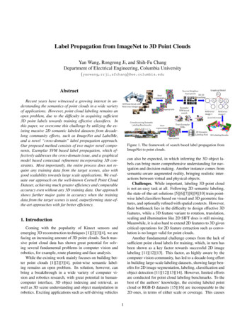
Algorithm 1: Building Superpixel Labeling Pool.123456Input: A set of superpixels with ground truth labelsS {Si , li }Ni 1for Superpixel Si S doTrain an Exemplar SVM for each superpixel withEquation 2 and hard negative miningendLearn a reranking function by solving Equation 5Output: A set of Exemplar SVMs with reranking(r)(r)weights and associated labels {wi , bi , wi , bi , li }Figure 2. Examples of search based label propagation from ImageNet [12] to Cornell Point Cloud Dataset [6]: (a) outputs fromNaive kNN, (b) outputs from ESVMs. We can see Naive kNN haslots of false positives (with red borders), e.g., it outputs printerand table for the input of wall. But ESVM performs much morerobust. For each result, we show not only the superpixel but alsoits surroundings for clarity.least distance D from Sq , and D(·, ·) is the metric usedto measure the distance among superpixels, e.g., Euclideandistance in the feature space.Propagation with Exemplar SVM. As pointed out in[18], nearest neighbor search with Euclidean distance cannot capture the intrinsic visual similarity between superpixels, while on the other hand training a label classifier is toosensitive to the training data, with large generalization erroragainst propagation.To address this issue, Exemplar SVM (ESVM) [18] isintroduced to build a robust metric. For every superpixelextracted from the labeling pool Si S, we train a linearSVM to identify its visually similar superpixels. The Exemplar SVM for Si is trained to optimize the margin of theclassification boundaries:1arg min kwi k22 C wi ,bi 2Xξj C {j yj 0}X{j yj 0}ξj ,(2)s.t. yj (wiT xj bi ) 1 ξj , j,where xj is the visual features extracted from Sj .To further guarantee the matching robustness, every superpixel Si is translated and rotated to expand to more positive examples for training. And the negative examples aresubsampled from other superpixels. Larger penalties C are given for false negatives to balance the boundary. However, even with this C setting, if a superpixel other than butvery similar to the exemplar appears in the negative set, itwill significantly degenerate the performance with an illtrained SVM, while this is not studied in object detection[18]. To address this issue, we add an extra constraint thatonly superpixels with different labels from Si can be chosenas negative examples.Hard Negative Mining. Different from regular Exemplar SVMs only able to find nearly identical instances, weset a small C in the training process for better generality, allowing examples not exactly the same as the exemplar alsohave positive scores. However, this may increase the number of false positives with different labels. To address thisproblem, given the decision boundary is only determined bythe “hard” examples (the support vectors), we introduce thehard negative mining to constrain the decision boundary:1. Apply the ESVM trained from Si on the training data,collecting the prediction scores {sj }2. Add the false positives {Sj sj 0, l(Sj ) 6 l(Si )}into the negative examples and launch another roundof SVM training3. Repeat the first two steps until no new hard examplesare found or a preset iteration number is reached.By the combination of small C and supervised hard negative mining with labels, we achieve a balance of generality and sensitivity. Figure 2 shows a comparison betweenESVM and naive kNN search. We can see that althoughnaive kNN usually outputs visually similar instances, it isnot robust against false positives, while ESVM does betterin label robustness, with more sensitivity on the differenceof labels.To label the superpixel Sq in the reference images, wefind the superpixels with the k strongest responses fromtheir ESVMs as its k nearest neighbors in S, i.e.,kkNN(Sq ) arg max Fi (wiT x(Sq ) bi ).Si S(3)Here Fi is the ranking function as introduced below.Learning Reranking Functions. While we use the relative ranking of SVMs’ prediction scores for kNN search,this relative order is still not constrained in the training process. We address this issue by learning a linear function foreach SVM for reranking, which minimizes the ranking erroramong different SVMs, i.e.,(r)Fi (x) wi(r)· x bi .(4)
Figure 3. Construction of the graphical model. (a) shows how to construct nodes and edges from an example point cloud. (b) shows theabstract representation of the graphical model, where N (Sj ) denotes the spatial adjacent superpixels of Sj in the reference images. And(c) shows the expected output after optimizing on the model. For clarity, only part of the connections are plotted in (a).This linear mapping does not modify the relative order ineach ESVM, but rescales and pushes the ESVMs jointlyto make their prediction scores comparable. This differsfrom the calibration step in [18] that transforms the decisionboundary of each SVM independently for object detection.More specifically, given a held-out superpixels validation set with ground truth labels SH {Sq }Hq 1 , we firstapply the ESVMs to get prediction scores {sq }Hq 1 , and thencollect SVMs with positive scores for reranking, only someof which have the same label with Sq . Here we aim to learnthe function Fi for each ESVM in S, making superpixelswith the same label as Sq have larger score than others, formulated as a structured learning-to-rank problem [23].minX1i2kwk22 CXξi,j,ks.t. for every query qi ,wT Φ(qi , sj ) wT Φ(qi , sk ) 1 ξi,j,k(5) l(Sj ) l(Sqi ), l(Sk ) 6 l(Sqi )ξi,j,k 0.Here w {(wi , bi )}ni 1 . Φ(qi , sj )’s (2j 1)th and 2jthdimensions are sj and 1 respectively, to encode the weightsand scores into a single vector. Although this problem is notconvex or differentiable, its upper bound can be optimizedefficiently with a cutting plane algorithm [24]. Algorithm 1shows the training procedures of our label propagation.3. 3D Contextual RefinementGiven the k nearest neighbors of each superpixel in thereference images, the next step is to label the point cloud{l(pi ) pi P} by backprojecting and fusing their labels.Considering a point pi in P may appear in different reference images with different viewing angles, our predictionexploits both the intra-image 2D context and the inter-image3D context, as shown in Figure 3. Note different from traditional contextual refinement approaches [5][6][25], our approach does not require any labeled 3D training data.Graphical Model. First the point cloud is oversegmented based on the smoothness and continuity [5], producing a 3D segment set {Di } as shown in Figure 3 (a).Second, with the transform matrices {Mi } from local 2Dcoordinates in reference images {Ii }Ri 1 to the global 3Dcoordinates, segments in {Di } are matched to the referenceimages, each resulting in a 2D region SMj (Di ). If this projected region shares enough portion with some superpixel{Si } from this reference image, we connect an edge between {Si } and SMj (Di ), as shown as red links in Figure 3(a). Spatially adjacent superpixels within one reference image are also connected, as shown as yellow links in Figure 3(a). Then, an undirected graph G {V, E} is built with 3Dsegments and 2D superpixels as nodes V {Di } {Sq }Mq 1and the connections mentioned above as edges E. Figure 3(b) shows the corresponding graphical model.For every node v, we adopt its label l(v) as the variableson the graphical model, and define the potential functionto enforce both intra-image and inter-image consistency, asdetailed later. In the end, the semantic labels L for 3D segments {Di } is inferred by minimizing the potential functionof the graphical model:arg minnL LXv V log ψd l(v) λX log ψs l(v1 ), l(v2 ) ,(v1 ,v2 ) E(6)in which L is the label set, n is the number of nodes in thegraphical model, and λ is a constant that weights differentpotential components. The potential function consists of thedata term ψd and the smoothing term ψs .The assigned labels of 2D superpixels are encouraged tobe the same as their results from label propagation. Therefore the data term is defined as, ψd l(Si ) exp pSi l(Si ) ,(7)where pSi (·) is the label distribution among kNNs of Siretrieved using Equation 3.Intra-Image Consistency. To encode the intra-imageconsistency in the reference images, neighbor superpixels
Algorithm 2: Search based Label Propagation.12345678Input: Point cloud P with reference images IR , andsuperpixel propagation pool SDo over-segmentation on both P and IRfor Superpixel Sq IR doUse Equation 3 to retrieve kNN from SendUse the over-segmentation structure of P and IR , andthe kNN of Sq to construct the graphical model asintroduced in Section 3Solve the graphical model by minimizing Equation 6with Loopy Belief PropagationOutput: 3D-segment-wise semantic labels of Pare encouraged to have related labels, defined by the intraimage smoothing term ψs,2D . ψs,2D l(Si ), l(Sj ) p l(Si ), l(Sj ) ,(8)in which p(·, ·) is the co-occurrence probability learnedfrom the superpixel labeling pool S.Inter-Image Consistency. To make the 3D labeling results consistent among reference images, we further definethe inter-image smoothing term as,( 1 l(Si ) l(Dj )ψs,3D l(Si ), l(Dj ) (9)c l(Si ) 6 l(Dj ),in which c 1 is a constant. Overall, we have a morespecific potential function design.X log ψ(L) log ψd l(Sq )Sq IRX λ1log ψs,2D l(Si ), l(Sj ) (Si ,Sj ) E,Si ,Sj IR λ2X log ψs,3D l(Si ), l(Dj ) .(Si ,Dj ) E(10)Similar with above, λ1 and λ2 denote the weights for different potential parts. We use Loopy Belief Propagation (LBP)to find a local minima of ψ. Algorithm 2 outlines the overallprocedure based on the potential design above.Integrating Other Contexts. If 3D point cloud training data with ground truth label is also available, we canfurther integrate stronger context into our graphical model.Such contexts may include 3D relative positions (e.g., a table may appear under a book but should not under floor),and normal vector (e.g. a wall must be vertical and floormust be horizontal), etc., as investigated in [5]. However,this requirement puts stronger dependence on training datathus decreases the generality.Figure 4. Superpixel distribution of the labeling pool (blue) andreference images (red) in the (dimension reduced) feature space.4. Experimental ValidationsData Collection. To build the superpixel labeling pool,we collect superpixels from ImageNet [12], which providesobject d
Manual point cloud labeling is certainly one solution to the lack of sufficient training data. However, it requires intensive human labor, especially considering the difficulty in labeling 3D points. Even given sufficient point cloud labels, the effective 3D feature design still remains open. But turning