Transcription
Journal of Statistics Education, v17n1: António Teixeira, Álvaro Rosa a.1 of xeirapdf.htmlStatistical Power Analysis with Microsoft Excel:Normal Tests for One or Two Means as a Prelude toUsing Non-Central Distributions to Calculate PowerAntónio Teixeira, Álvaro Rosa and Teresa CalapezIBS – ISCTE Business School (Lisbon)Journal of Statistics Education Volume 17, Number 1 ira.htmlCopyright 2009 by António Teixeira, Álvaro Rosa and Teresa Calapez, all rights reserved. This text may befreely shared among individuals, but it may not be republished in any medium without express written consentfrom the authors and advance notification of the editor.Key Words:Effect size; Excel; Non-central distributions; Non-centrality parameter; Normal distribution; Power.AbstractThis article presents statistical power analysis (SPA) based on the normal distribution using Excel, adoptingtextbook and SPA approaches. The objective is to present the latter in a comparative way within a frameworkthat is familiar to textbook level readers, as a first step to understand SPA with other distributions. The analysisfocuses on the case of the equality of the means of two populations with equal variances for independentsamples with the same size.This is the situation adopted as case 0 by Cohen (1988), a pioneer in the subject, to develop his set of tables andso, the present article can be seen as an introduction to Cohen’s methodology applied to tests based on samplesfrom normal populations. We also discuss how to extend the calculation to cases with other characteristics(cases 1 to 4), similarly to what Cohen proposes, as well as a brief discussion about the advantages andshortcomings of Excel. We teach mainly in the area of business and economics, which determines the scope ofour analysis.1. IntroductionIf you browse a sample or even the universe of textbooks of statistics applied to business and economics, youwill most surely see references to the calculation of the power of statistical significance tests only when thenormal distribution is used (Berenson and Levine, 1996; Bernstein and Bernstein, 1999; Freund, 1962; Kazmierand Poll, 1979; Levin and Rubin, 1998; Levine et al., 1999; Pestana and Velosa, 2002; Pinto and Curto, 1999;Reis et al., 2001; Sanders, 1990; Sandy, 1990; Smithson, 2000; and Spiegel, 1972). Watson et al., 1993 presentthe subject as optional, while Webster (1998) and Berenson and Levine (2004) only explain the concept withoutgiving any examples. The calculation of the minimum sample size that guarantees predefined values for alphaand beta is a main subject in only three of the above references (Berenson and Levine, 1996, Kazmier et al.,2/26/2009 1:59 PM
Journal of Statistics Education, v17n1: António Teixeira, Álvaro Rosa a.2 of xeirapdf.html1979 and Smithson, 2000), while a fourth (Freund, 1962) presents the formula, asking for its deduction as anexercise. In brief terms, SPA does not get the importance it deserves in these books.The cause of this situation is most surely the fact that the extension of SPA involves an additional set of(non-central) distributions and a greater number of tables. The panorama is not exactly the same in the socialsciences where the greater importance given to the subject can be explained by the American PsychologicalAssociation (APA) requirements (Kline, 2004; American Psychological Association, 1994 and 2001).As Smithson (2002)alleges when talking about a similar subject (confidence intervals with non-central distributions), "prior to thewide availability of computing power, exact confidence intervals for the proportion for small samples werepainstakingly hand-calculated and tabulated. Confidence intervals whose underlying sampling distributions arenot symmetrical and not a constant shape were labor intensive and impractical without computers, so they were(and still are) neglected in textbooks and, ironically, popular statistical computer packages." For example, inwhat concerns SPA, SPSS Inc offers a product that is independent of the SPSS application itself, Sample Size.We intend to fill this gap by presenting an integrated analysis with a common language that will allow thedevelopment of a set of tools to be used knowingly by students and practitioners, giving them a path to thinkabout the problem and to analyze results produced by others, eliminating the pure automation involved inobtaining numbers by pressing a key in the computer keyboard, or avoiding what Pestana and Velosa (2002) callturning off their heads when turning on the computer. With the advent of computers and the generalization of itsuse, computation limitations are something from the past. Excel has the capacity to implement these models.The necessary capabilities that are not built in can be created through user defined routines. It is not certain thatexact results are always obtained but Excel is a privileged tool for students to perform and follow the severalsteps involved in the situations under consideration.When designing a course we must be aware that students can have in their future professional lives two levels ofcontact with the subjects taught. One refers to performing statistical analyses and the other reading those madeby others. The teacher must not consider courses with closed borders. Doors must be opened, allowing insightsinto things beyond the course limits. As we teach at graduation and post-graduation levels, we have beenconfronted with many cases of students declaring "now I understand what you really meant when saying ." Ifno such doors exist, crossing to wider perspectives is more difficult.Understanding Cohen’s framework leads to understanding the effect size approach widely used in the socialsciences. Even if students will never use this methodology, they may be exposed to it when reading analysesperformed by others. Additionally, they may be exposed to it, especially in the fields of the social sciences, incourses like research methods. We consider that teachers who have such students in their classes might find ithelpful for thinking about how to present power analysis in class.Although table based teaching introduces limitations to the domain to be covered and in some cases returnsdiscrete information about a continuous underlying distribution, we decided to conduct this first approach inparallel with the tables created by Cohen (1988). In this way, the present article is an introduction to Cohen’smethodology applied to tests based on samples from normal populations. It could be seen as "the chapter thatCohen (1988)did not write" or a preamble to a better understanding of his work. Our methodology will then show how onecan easily construct Cohen-like tables using Excel. Besides constituting a tribute to Cohen’s pioneer work, wealso believe this is the best way to convey the knowledge at the level we want at this stage, which is tounderstand the methods involved and the tools available instead of supplying automated solutions subject to the"garbage in garbage out" perils. We do not intend to follow the instant pudding route. Even if the user has accessto software applications that will directly give the desired results, we intend to arm him with enough knowledgeand alternative routes to check those results by performing the calculation process step by step.2/26/2009 1:59 PM
Journal of Statistics Education, v17n1: António Teixeira, Álvaro Rosa a.3 of xeirapdf.htmlTables can also be seen as a base for charting results. In this specific case, there is a wide range of combinationsof inputs and formulas to use. When comparing functions and routines used, these tables define what we can calla Cohen’s universe, fixing borders. We can confine accuracy analyses to this universe, especially when dealingwith the subject for teaching purposes.Furthermore, computing power directly does not replace the use of tables in teaching. Instead of static tables wecan have applications that will reformulate the tabulated values each time entry values are changed. Forexample, in SPA, the teacher can generate problem-specific tables and include them in examination papersinstead of generic tables that would require a large variety of entries. This kind of models and reasoning tends toassume a more important role, as classes - and even examinations – are becoming more and more lab based. Theconstruction of tables is also a good exercise for students to become familiar with the characteristics ofstatistical distributions.As this article is Excel based, we also include a section about software limitations, somewhat beyond the scopeof this specific article, in order to create a centralized reference to this matter to be used in forthcoming work.This article is just the first of a series about power and precision analysis. The concentration of theseconsiderations helps to confer unity to the set of final articles.To avoid unnecessary extension of the article, we assume that the reader is familiar with concepts such as type I(alpha) and type II (beta) errors, structure of hypotheses testing and the power (pi) of a test, avoiding the need toexplain them in detail. The meaning of all symbols used can be found at the end of the article. This results in amore compact and easier to read article.2. Excel Advantages, Shortcomings, and OdditiesThe wide use of Excel is the main reason for its choice. It is a tool familiar to most users for the development ofmodels related to a wide range of scientific and practical fields. Despite the limitations we are identifying here,it is an excellent tool for teaching purposes, allowing students to shed light into what can otherwise be seen asblack boxes. With Excel one can learn while performing all calculation steps and easily creating graphicalrepresentations. On the other side, the shortcomings we are listing emphasize the necessity of analyzingcritically computer generated results even in applications that are considered as more reliable.There are two eras concerning the use of Excel for statistical analysis: pre and post Excel 2003. In his review ofExcel 2003, Walkenbach (2008), referring to what Microsoft indicates as enhancements in the statisticalfunctions, states: "This, of course, is a new definition of the word enhancements. Truth is, these functions havebeen broken for more than a decade, and they finally return accurate results in Excel 2003."Knüsel (1998, 2002, 2005) has been studying the accuracy of Excel statistical functions and considers that"some of previously indicated errors in Microsoft Excel 97 and Excel XP have been eliminated in Excel 2003.But some others have not been corrected and new ones have been found ". Sleeper (2006) approaches thissubject in a subchapter named Defects and Limitations of Microsoft Excel Spreadsheet Software where hepresents a list of problems either solved or remaining in Excel 2003, indicating that he still found the latter in thebeta version of Excel 2007. We have checked the cases indicated in Knüsel (2005) and found that nothing haschanged in the release version.In statistical terms the remaining problems concern the accuracy of statistical functions in part of their domain,namely, using Excel designations, in RND (in what concerns the random number generator), POISSON,BINOMDIST, CHIINV, GAMMADIST, BETAINV, and NEGBINOMDIST.Sleeper (2006)also refers to the ill-functioning of Excel’s QUARTILE and PERCENTILE functions. It is not quite so. As2/26/2009 1:59 PM
Journal of Statistics Education, v17n1: António Teixeira, Álvaro Rosa a.4 of xeirapdf.htmlLarson and Faber (2000)acknowledge, there are several ways of finding the quantiles of a data set. Instead of the most usual formulas tocalculate the position of the first and third quartiles, (n 1)/4 and 3 (n 1)/4, Excel uses (n 3)/4 and (3n 1)/4respectively. These seldom appear in textbooks but can be found, for instance, in Murteira et al. (2002). Themethod should be included in the help file to avoid misinterpretations.Another shortcoming we did not find reported is the lack of ability to detect multimodal data: the MODEfunction, given any data set, returns only one value. The problem is that, for multimodal data, the value reportedmay vary upon sorting.As a conclusion Sleeper (2006)acknowledges that for statistical calculations Excel 2003 and later are not perfect but acceptable, recommendingthat the Analysis Toolpak add-in provided with any version of Excel should never be used, giving as referencethe Microsoft Knowledge Base Article to get a detailed view of the problems involved (Microsoft, 2007), takinginto account that some of them have been improved.Besides the limitations indicated above there is a wider set of oddities, some of them presented by Walkenbach(2008)regarding the sum of Boolean values. We also found that validation of input does not work when using the PasteSpecial alternative. Microsoft (2007a, 2007b) elaborates about problems involving floating-point arithmetic andhow to remedy them.Whenever a new application is developed bugs tend to appear. Nevertheless, Excel is a valuable and versatiletool to accomplish a wide range of objectives including the one we are pursuing: to teach statistics.3. Statistical Power Analysis with the Normal Distribution UsingMicrosoft ExcelThere are several different situations involving the tests for the mean of one or two populations. Cohen (1988)considers those indicated in Table 1.Table 1 ‐ Tests for means included in Cohen (1988)Case 0Case 1Case 22 means; σa σb ; na nb2 means; σa σb ; na nb2 means; σa σb ; na nbCase 3Case 41 sample size n2 paired observations in a sample size nHe develops the tables for case 0, although they can also be used for the other cases provided some additionalcalculations are made to find the tables’ input values. Consequently, we will deal with this case as the basesituation. The tests can also be one tailed (upper or lower) or two tailed. Cohen presents tables for two and oneupper tailed tests (obviously, the latter will allow the calculation of power of one lower tailed test). All the othercases can be transformed into one of these two. It is notable that Cohen leaves aside the case in which σa σb ;na nb. We will also ignore it for now, leaving its consideration for future work on power and precision whiletesting means.2/26/2009 1:59 PM
Journal of Statistics Education, v17n1: António Teixeira, Álvaro Rosa a.5 of xeirapdf.htmlDue to its similarity, we will deal only with two tailed tests, using the upper tail to calculate the power. The casewe consider is then the one on the left in Table 2, where Hp and μp refer to the values of the mean to use whencalculating power. This restriction does not affect the generality of the conclusions.Table 2 - Type of tests considered by CohenTwo TailedUpper TailedThe test statistic can be either the sample meanor its standardized valuein the case of one populationwhereas in the case of two populations, it can be the difference between the two sample meansor itsstandardized value. Textbooks show both, standardized and non-standardized, to arrive at a decision, but the value of the type IIerror, beta, is calculated (almost always) using the non-standardized test statistic. It happens that Cohen’smethodology asks for the opposite, that is, the use of the standardized value.In any case, the test is carried out by defining a rejectionand a non-rejectioninterval that are expressedin terms of the statistic used for the test. As we will calculate power as π 1 β, we are concerned with ,which is defined in Table 3. Note that we are using ]a;b[ for an open interval, [a;b] for a closed one, and everymixed situation accordingly with these.Table 3 – Rejection and non-rejection regionsTest StatisticTwo TailedUpper TailedUnstandardizedStandardizedWe can approach power from two perspectives: (1) a posteriori: calculating the power after performing the test;(2) a priori: calculating the sample size needed to obtain a minimum desired value for power, as well as foralpha. Additionally, we will consider only the cases in which the finite population correction factor for thecalculation of the standard error is not necessary.3.1 Computation of Power Using the Usual WayAs an example of calculating power for the two tailed test alternative, we will use the specific situationpresented in Table 4.2/26/2009 1:59 PM
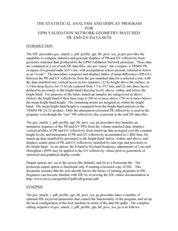
Journal of Statistics Education, v17n1: António Teixeira, Álvaro Rosa a.6 of xeirapdf.htmlTable 4 – Example considered in the analysis of power calculationAn investor is interested in testing the hypothesis that the mean householdmonthly income is the same in two metropolitan areas. For this purpose, astatistical consultant performed a survey using two independent simplerandom samples with the same size:following results for the mean of each sample:, obtaining the.From the results of previous studies, the consultant assumes that thestandard deviation of the household incomes in both areas is the same:The valueis used for the statistical significance of thetest. The alternative value of the difference between the two means forcomputing the power of the test is3.1.1. Power Computation a posterioriThe usual way of performing this test usingas the test statistic leads to the results presented in Table5. Putting aside for now the calculation of beta, the decision is taken based on the assumption that H0 is true, i.e.there is no difference between the two population means. From Table 5 we can see that the test statistic belongsto the non-rejection interval, leading to the non-rejection of H0.Table 5 – Performing the test usingas the test statisticDecision: do not reject H0The probability of committing a type II error (beta) is associated with the non-rejection interval of the normalcurve represented at the left on Figure 1. However, when computing the type II error, the falsity of H0 isassumed, meaning that we can no longer work with a normal distribution with μ0 (μa μb)H0 0.2/26/2009 1:59 PM
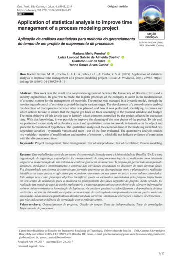
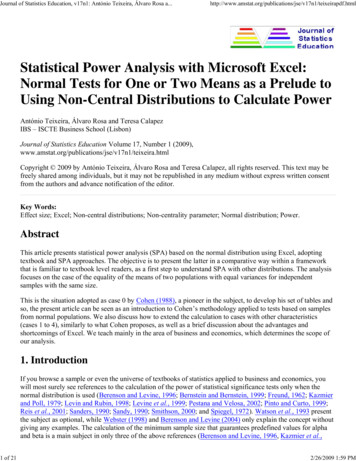
Journal of Statistics Education, v17n1: António Teixeira, Álvaro Rosa a.7 of xeirapdf.htmlTherefore, the calculation of power needs specification of alternative values for the difference between the twomeans. The situation can be dealt (as we do in this case) either with the consideration of a point value indicatedin Hp, or by constructing a power function for several alternative values for the mean. We followed the formerbecause the later is just a repetition of the procedure presented.Type I error (alpha) is represented by the darker (blue) shaded area in Figure 1 and Type II error (beta) by thelighter (grey) shaded area, with valueThe power of the test, π 1 - β 0.89, is represented by the brown area in Figure 1.Figure 1 – Graphical representation of alpha, beta and powerFigure 2 shows how this value can be easily obtained using the functions embedded in Excel. Please note that inthe Excel sheets pictured, grey background cells correspond to inputs, white background cells to intermediateresults and inverse background (yellow over blue) cells to final results.Figure 2 – Computation a posteriori of power using Excel formulas and embedded functions3.1.2. Power Computation a prioriThe a priori computation of power is the determination of a sample size n guaranteeing that pre-defined valuesfor alpha and beta will not be exceeded. Let us suppose that we want to test the equality of the population meansin a way that the values of alpha and beta will not be greater than 0.05 and 0.10 respectively. Figure 3 illustratesthe base from which we can derive a for
Excel 2003, Walkenbach (2008), referring to what Microsoft indicates as enhancements in the statistical functions, states: "This, of course, is a new definition of the word enhancements. Truth is, these functions have been broken for more than a decade,