Transcription
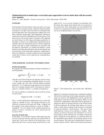
Optimization driven model-space versus data-space approaches to invert elastic data with the acousticwave equationXiang Li , Anaı̈s Tamalet , Tristan van Leeuwen , Felix J.Herrmann EOS-UBCInverting data with elastic phases using an acoustic wave equation can lead to erroneous results, especially when the numberof iterations is too high, which may lead to over fitting the data.Several approaches have been proposed to address this issue.Most commonly, people apply “data-independent” filtering operations that are aimed to deemphasize the elastic phases in thedata in favor of the acoustic phases. Examples of this approachare nested loops over offset range and Laplace parameters. Inthis paper, we discuss two complementary optimization-drivenmethods where the minimization process decides adaptivelywhich of the data or model components are consistent withthe objective. Specifically, we compare the Student’s t misfitfunction as the data-space alternative and curvelet-domain sparsity promotion as the model-space alternative. Application ofthese two methods to a realistic synthetic lead to comparableresults that we believe can be improved by combining thesetwo methods.equal to 0.25. As we can see in Figure 1(a) and Figure 1(b),the elastic data contain elastic phases that are not present inthe acoustic data. These elastic phases are not modelled by theacoustic wave equation and will thus affect the recovery as wecan see by comparing Figures 2(a) and 0006000800010000(a)0TIME-HARMONIC ACOUSTIC FWI FORMULATION0.5Problem formulationWe consider the following frequency-domain formulation ofthe FWI problem:1.5min φ (m, w) m,wKXs122.5ρ(B i (di wi F i (m)),(1)3i 13.5where di is the observed data for one frequency and one sourcei, F i (m) is the corresponding modelling operator, w are thesource weights, m is the vector with the unknown mediumparameters, B i is a data-processing operator (to be discussedlater), ρ is a penalty function and K is the batch size which isequal to ns (number of shots) n f (number of frequencies).For a given model m, we estimate the source wavelet by solvingfor each source:minimize ρ(B i (di wi F i (m))).wi(2)This is a scalar optimization problem that can be solved efficiently in a number of ways. The objective function is noweffectively a function of the model only: φ (m) φ (m, w) andthe gradient of the reduced objective is given by φ (m) m φ (m, w). For more details on this variable projection approach, we refer to (Aravkin et al., 2012; Aravkin and vanLeeuwen, 2012)Inversion of elastic dataIn this paper, we use the BG compass model depicted in Figure 3(a) as the true reference and carry out acoustic FWI onelastic data. The S-wave velocity for the elastic data is computed from the P-wave velocity using a fixed Poisson’s ratio4020004000m(b)Figure 1: Time-domain data. (a) Acoustic data. (b) Elasticdata.Opposed to commonly used data-space continuation methods,which involve nested loops where Laplace parameters and offsetranges are chosen to first highlight the acoustic and then theelastic phases in the data (Virieux and Operto, 2009), we willconsider two complementary optimization-driven approaches tomitigate the affects of ignoring elasticity in the forward model.In the first approach, the missing elastic phases are seen asoutliers, whose adverse imprint on the inversion is controlledby using the Student’s t misfit function. This type of datamisfit function is known to be insensitive to outliers. Theseartifacts are known to become more dominant if we run toomany iterations, which will lead to an “over fitting” of the elasticphases. During the second approach, we control the affects ofthe unmodelled elastic phases by promoting sparsity in thecurvelet domain. This latter type of regularization is known topenalize spurious artifacts. Before discussing the performance
Optimization driven 0regularize updates in the model space. For this purpose,P wedefine the data-misfit via the least-squares–i.e., ρ(r) i ri 2 ,where r is the data residual vector as defined before. Contraryto Student’s t, we impose 1 -norm constraints on the curveletrepresentation of the Gauss-Newton updates (Li et al., 2012),i.e., we solve the following modified Gauss-Newton problems:1δ m CH arg min kδ D diag(w) F [m0 ]CH xk2F2xsubject to kxk1 400050006000700080009000100001500(b)Figure 2: Acoustic FWI results (a) On acoustic data. (b) Onelastic data.of these two approaches, let us first briefly describe these twomethods.Data-space Student’s tAs shown in (Aravkin et al., 2011), the Student’s t penalty isgiven byXρ(r) log(1 ri 2 /k),(3)iithwhere ri is thedatum of the residue vector given by thedifference between the observed and modelled data, and k isthe degree of freedom of the Student’s t distribution.This misfit function can be used in FWI in order to improve therecovery in the presence of large outliers or unexplained eventsin the data. Indeed, in contrast to previous robust penalties,the Student’s t penalty is non-convex. Thus, large outliers areprogressively down-weighted and effectively ignored once theyare large enough.However, for the Student’s t penalty to be effective, the outliersmust be somehow localized and distinguishable from the gooddata. Thus, following (van Leeuwen et al., 2013), we first transform the residual into a domain where the outliers are localizedvia the processing operator B i before measuring the Student’st misfit. We can use any transform that would normally be usedto filter out the noise (Fourier for periodic noise, Radon fornoise with moveout, Curvelets for more complicated coherentevents, etc.). Here, we choose to transform the residual in thesource-receiver wave-number domain by applying the Fouriertransform along both the sources and the receivers. The advantage of this approach is that the optimization with the Student’st misfit carries out the filtering adaptively rather than relying onsome user-defined prior filter. So, we let the robust inversionprocess decide which parts of the data can be fitted and whichshould be ignored. Thus, the filtering is done implicitly as partof the inversion process.Model-space sparsity promotionAside from controlling the inversion via the Student’s t misfitfunction in the data space, another possible approach is tofor a series of increasing τ’s. In this expression, the symbol CHstands for the curvelet synthesis given by the adjoint, denoted byH , of the curvelet transform. The data-residue matrix is given byδ D D diag(w)F (m0 ), with D [d1 , d2 , d3 , · · · , dK 0 ] theobserved data for randomly selected sources and frequencies.Since K 0 Ks, the evaluation of the Jacobian diag(w) F [m0 ],scaled by the source weights w, becomes cheaper making thesolution of Equation 4 computationally feasible (Herrmannet al., 2009, 2008; Li et al., 2012). Following the modifiedGauss-Newton approach, we compute the 1 -norm constraintsviakδ Dk2τ (5)kC F T (m0 )diag(w)δ Dk (Berg and Friedlander, 2008).EXPERIMENTSTo make a comparison between data-space Student’s t andmodel-space sparsity promotion, we use the BG compass modelin Figure 3(a) as the true reference, which is a synthetic P-wavevelocity model created constrained by real well-log information.As we mentioned before, we compute the S-wave velocity(Figure 3(b)) using a fixed Poisson’s ratio of 0.25. We simulate101 shot records with a 100m interval using a time-domainelastic finite-difference modeling code (Thorbecke, 2013) witha 9Hz Ricker wavelet. All shots share the same 401 receiverswith 25m interval yielding a 10km offset. Because we consideran ocean-bottom node survey with reciprocity, we set the sourcedepth to 200m while receiver depth is set to 10m.The modeling kernel used in the inversion is based on frequency domain acoustic modeling implemented by solving theHelmholtz system for a 9-point stencil (Jo et al., 1996). Todefine the starting model for the inversion, we smooth and average laterally the reference velocity model in Figure 3(a). Theresult is plotted in Figure 3(c).To make a fair comparison, both inversions are carried out withmultiple frequency bands from 3 20Hz. Each frequency bandcontains 3 frequencies. For data-space Student’s t, we compute5 and 10 l-BFGS updates with all the sources while for modelspace sparsity promoting, we solve 5 sparsity-promoting GNsubproblems with 50 randomly selected shots. For 5 iterationsof l-BFGS, the total number of PDE solves is roughly thesame for these two approaches. We varied the number of lBFGS iterations to show the effect of overfitting (juxtaposeFigures 4(a) and 4(b)).As we have seen from the motivating example in the introduction, carrying out acoustic FWI on data that contain elas-
Optimization driven 00700080009000100001500(c)Figure 3: BG compass model. (a) True P-wave model. (b) TrueS-wave model. (c) Initial model.tic phases can be detrimental to the inversion. Using the robust Student’s t technique, we hope to mitigate some of theadverse affects of these elastic phases by using the fact thatmonochromatic frequency slices are relatively sparse in thesource-receiver wave-number domain. This means that the elastic events that are not in the range of the acoustic modelingoperator tend to be concentrated amongst a limited numberof frequencies. The Student’s t penalty function is by designrelatively insensitive to these outlliers. which should improvethe inversion results. As we can see from Figure 4(c), this isindeed the case compared to the inversion result based on the 2misfit for 10 iterations included in Figure 4(b). While this resultmay not be as good as the inversion result for the acoustic onlyresult, our improvement is certainly encouraging. Aside fromchanging the data-space misfit penalty functional, model-spaceregularization is another proven tool in inversion problems thatsuffer from null spaces or from unmodelled noise. Transformdomain sparsity promotion, including one-norm minimizationin the curvelet domain, has proven to be an effective tool toremove these unmodelled signal components. For this purpose,we submit the data set with the elastic phases to the above described modified Gauss-Newton method. The results of thisexercise are summarized in Figure 5 and were obtained by 5GN iterations on randomized subsets of 50 shots. From thisfigure, it is clear that invoking curvelet-domain sparsity promotion on the GN updates also mitigates the adverse affectson the unmodelled elastic phases present in the data. Whilethe Student’s t approach works by ignoring the outliers, thecurvelet-domain sparsity promotion penalizes complexity onthe model that is associated with the unmodelled elastic 0001500(c)Figure 4: l-BFGS inversion results. (a) Least-Squares penaltywith 5 iterations. (b) Least-Squares penalty with 10 iterations.(c) Student’s t penalty with 10 iterations.As with the Student’s t, the result of this method is encouraging.DISCUSSION AND CONCLUSIONSWhile the results of the two different methods are encouraging,there is still room for improvement. Before outlining a possibleroad ahead let us first systematically compare the results ofthe previous two sections. Upon close inspection, the resultobtained with the Student’s t penalty function has more detailscompared to the results obtained by GN but also more artifactsrelated to the presence of elastic phases. When we comparevanilla l-BFGS (Figure 4(b)) without Student’s t with the vanillaGN (Figure 5(a)) without curvelet-domain promotion, we observe that the result for GN are apparently less sensitive tounmodelled phases in the data.From the computational perspective, the Student’s t approachis relatively simple since it relies on more-or-less straightforward changes on the definition of the penalty function itself(compared the commonly used 2 penalty), its gradient, and theestimation of the Student’s t parameter by variable projection.The modified Gauss-Newton approach, on the other hand, relieson a somewhat more complicated machinery that includes thecurvelet transform itself and a method to choose the 1 -normconstraint for each GN subproblem. The advantage of the GNapproach, however, is that it does not rely on computing thegradients for all shots as required by the Student’s t method,
Optimization driven FWI45000400050035001000300025001500 1 -norm constraint can be relaxed without running the risk offitting the elastic events, which are, by virtue of the Student’s tpenalty, 080009000100001500(b)Figure 5: Gauss-Newton inversion inversion results. (a) GNwithout sparsity promoting. (b) GN with sparsity promoting.which relies on Fourier transformation along the fully-sampledsource and receiver coordinates. Moreover, elastic phases represented as monochromatic frequency slices may not be optimallysparse in the Fourier domain, which jeopardizes our ability toseparate the acoustic from the elastic phases using the Student’st. This failure to completely separate the acoustic and elasticphases is properly responsible for the remaining artifacts forthe Student’s t (cf. Figure 4(c)). The GN is more artifact freebut this feature goes at the expense of loss of detail, which isrelated to the one-norm constraint and perhaps the number ofiterations. If we relax the 1 -norm constraint too much, we runthe risk of starting to “over fit” the elastic events.As for the GN method, comparison between the vanilla l-BFGSand GN shows that the latter is apparently less sensitive tounmodelled phases in the data. There may be two possibleexplanations for this observation. First, the GN updates areregularized because we invert the GN Hessian with a limitednumber iterations, which corresponds to some kind of modelspace regularization. The l-BFGS, on the other hand, is notregularized. Second, l-BFGS attempts to invert the true Hessian via a low-rank approximation while the GN updates areobtained by (approximate) inversion of the GN Hessian formedby the composition of the adjoint of the Jacobian acting on theJacobian itself. In cases where the modeling operator does notexplain all the events in the data, it may not be reasonable toexpect that l-BFGS will yield the correct inverse of the Hessian while we can argue that the GN approach will at leastget the GN part of the Hessian correct if the velocity model isreasonably accurate.From our perspective, the results outlined in this abstract areboth encouraging and call for a joint formulation based on dataspace robust statistics in some transform-domain for the penaltyfunction and on model-space regularization, for instance viacurvelet-domain sparsity promotion, on the model updates. Themodified GN framework allows for this type of formulationsince it offers flexibility regarding the choice of the misfit function and norm on the model. In this way, we anticipate that theWe would like to thank the sponsors of the SINBAD project.This work was partly supported by a NSERC Discovery Grant(22R81254) and CRD Grant DNOISE II (375142-08).
Optimization driven FWIREFERENCESAravkin, A., T. van Leeuwen, and F. Herrmann, 2011, Robustfull-waveform inversion using the student’s t-distribution:SEG Technical Program Expanded Abstracts, 30, 2669–2673.Aravkin, A. Y., and T. van Leeuwen, 2012, Estimating nuisance parameters in inverse problems: Inverse Problems, 28,115016.Aravkin, A. Y., T. van Leeuwen, H. Calandra, and F. J. Herrmann, 2012, Source estimation for frequency-domain fwiwith robust penalties: Presented at the EAGE technical program, EAGE, EAGE.Berg, E. V. D., and M. P. Friedlander, 2008, Probing the Paretofrontier for basis pursuit solutions: Siam J. Sci. Comput., 31,890–912.Herrmann, F. J., C. R. Brown, Y. A. Erlangga, and P. P. Moghaddam, 2009, Curvelet-based migration preconditioning andscaling: Geophysics, 74, A41.Herrmann, F. J., P. P. Moghaddam, and C. C. Stolk,2008, Sparsity- and continuity-promoting seismicimaging with curvelet frames: Journal of Appliedand Computational Harmonic Analysis, 24, 150–173.(doi:10.1016/j.acha.2007.06.007).Jo, C. H., C. Shin, and J. H. Suh, 1996, An optimal 9-point,finite-difference, frequency-space, 2-D scalar wave extrapolator: Geophysics, 61, 529–537.Li, X., A. Y. Aravkin, T. van Leeuwen, and F. J. Herrmann,2012, Fast randomized full-waveform inversion with compressive sensing: Geophysics, 77, A13–A17.Thorbecke, J., 2013, 2d acoustic/visco-elastic finite differencewavefield modeling.van Leeuwen, T., A. Y. Aravkin, H. Calandra, and F. J. Herrmann, 2013, In which domain should we measure the misfitfor robust full waveform inversion?Virieux, J., and S. Operto, 2009, An overview of fullwaveform inversion in exploration geophysics: Geophysics,74, WCC1–WCC26.
Figure 1: Time-domain data. (a) Acoustic data. (b) Elastic data. Opposed to commonly used data-space continuation methods, which involve nested loops where Laplace parameters and offset ranges are chosen to first highlight the acoustic a
