Transcription
Programming Robots in ROSSlides adapted from CMU, Harvardand TU Stuttgart
Path Planning ProblemGiven an initial configuration q startand a goal configuration q goal, wemust generate the best continuous pathof legal configurations between thesetwo points, if such a path exists.
Illustration of Basic DefinitionsborderLegalconfigurationsq startobstaclesOptimalpathq goal
Feedback control, path finding, trajectory optim.path findingtrajectory optimizationfeedback controlgoalstart Feedback Control:E.g., qt 1 qt J ] (y φ(qt )) Trajectory Optimization:argminq0:T f (q0:T ) Path Finding: Find some q0:T with only valid configurations6/61
Control, path finding, trajectory optimization Combining methods:1) Path Finding2) Trajectory Optimization (“smoothing”)3) Feedback Controlpath findingtrajectory optimizationfeedback controlstartgoal Many problems can be solved with only feedback control (though notoptimally) Many more problems can be solved locally optimal with only trajectoryoptimization Tricky problems need path finding: global search for valid paths7/61
Types of Navigation Approaches Reactive (Purely Local) Visual Homing, Wall Following Bug-Based Algorithms Sense Direction and Distance to Goal Metric Path Planning Path Represented as a Series of Waypoints Assumes Distance-Based Map or Graph
Outline Bug Algorithms Artificial Potential Fields Wavefront Planning Visibility/Voronoi Graphs Configuration-Space (C-Space) Quad-Trees Probabilistic Road Maps
Buginner Strategy“Bug 0” algorithm known direction to goal otherwise local sensingwalls/obstacles & encodersGoal1) head toward goal2) follow obstacles until you canhead toward the goal again3) continueStartpath ?
Buginner Strategy“Bug 0” algorithm1) head toward goal2) follow obstacles until you canhead toward the goal again3) continueassume a leftturning robotThe turning direction mightbe decided beforehand OK ?
Bug ZapperWhat map will foil Bug 0 ?“Bug 0” algorithm1) head toward goal2) follow obstacles until you canhead toward the goal again3) continuegoalstart
A better bug?Call the line from the startingpoint to the goal the m-line“Bug 2” Algorithm1) head toward goal on the m-line
A better bug?Call the line from the startingpoint to the goal the m-line“Bug 2” Algorithm1) head toward goal on the m-line2) if an obstacle is in the way,follow it until you encounter them-line again.
A better bug?m-line“Bug 2” Algorithm1) head toward goal on the m-line2) if an obstacle is in the way,follow it until you encounter them-line again.3) Leave the obstacle and continuetoward the goalOK ?
A better bug?“Bug 2” Algorithm1) head toward goal on the m-lineStart2) if an obstacle is in the way,follow it until you encounter the mline again closer to the goal.3) Leave the obstacle and continuetoward the goalGoalBetter or worse than Bug1?
Outline Bug Algorithms Artificial Potential Fields Wavefront Planning Visibility/Voronoi Graphs Configuration-Space (C-Space) Quad-Trees Probabilistic Road Maps
The Basic Idea A really simple idea:– Suppose the goal is a point g 2– Suppose the robot is a point r 2– Think of a “spring” drawing the robot towardthe goal and away from obstacles:– Can also think of like and opposite chargesAdapted from slides by Howie Choset, with slides from Ji Yeong Lee, G.D. Hager and Z. Dodds
Attractive/Repulsive Potential Field– Uatt is the “attractive” potential --- move to the goal– Urep is the “repulsive” potential --- avoid obstaclesAdapted from slides by Howie Choset, with slides from Ji Yeong Lee, G.D. Hager and Z. Dodds
Artificial Potential Field Methods:Attractive PotentialConical PotentialQuadratic PotentialFatt (q) U att (q) k goal (q)Adapted from slides by Howie Choset, with slides from Ji Yeong Lee, G.D. Hager and Z. Dodds
Artificial Potential Field Methods:Attractive PotentialCombined PotentialIn some cases, it may be desirable to have distancefunctions that grow more slowly to avoid huge velocitiesfar from the goalone idea is to use the quadratic potential near thegoal ( d*) and the conic farther awayOne minor issue: what?Adapted from slides by Howie Choset, with slides from Ji Yeong Lee, G.D. Hager and Z. Dodds
The Repulsive PotentialAdapted from slides by Howie Choset, with slides from Ji Yeong Lee, G.D. Hager and Z. Dodds
Repulsive PotentialAdapted from slides by Howie Choset, with slides from Ji Yeong Lee, G.D. Hager and Z. Dodds
Total Potential FunctionU (q) U att (q) U rep (q)F (q) U (q) Adapted from slides by Howie Choset, with slides from Ji Yeong Lee, G.D. Hager and Z. Dodds
Potential FieldsAdapted from slides by Howie Choset, with slides from Ji Yeong Lee, G.D. Hager and Z. Dodds
Outline Bug AlgorithmsArtificial Potential FieldsWavefront PlanningVisibility/Voronoi GraphsConfiguration-Space (C-Space)Quad-TreesProbabilistic Road Maps
Computing Distance: Use a Grid use a discrete version of space and work from there– The Brushfire algorithm is one way to do this need to define a grid on space need to define connectivity (4/8) obstacles start with a 1 in grid; free space is zero48Adapted from slides by Howie Choset, with slides from Ji Yeong Lee, G.D. Hager and Z. Dodds
The Wave-front Planner Apply the brushfire algorithm starting from the goal Label the goal pixel 2 and add all zero neighbors to L– While L dequeue the top element of L, t set d(t) to 1 mint’ N(t),d(t) 1 d(t’) Enqueue all t’ N(t) with d(t) 0 to L (at the end) The result is now a distance for every cell– gradient descent is again a matter of moving to the neighbor with thelowest distance valueAdapted from slides by Howie Choset, with slides from Ji Yeong Lee, G.D. Hager and Z. Dodds
The Wavefront Planner: SetupAdapted from slides by Howie Choset, with slides from Ji Yeong Lee, G.D. Hager and Z. Dodds
The Wavefront in Action (Part 1) Starting with the goal, set all adjacent cells with “0” to the current cell 1– 4-Point Connectivity or 8-Point Connectivity?–Your Choice. We’ll use 8-Point Connectivity in our exampleAdapted from slides by Howie Choset, with slides from Ji Yeong Lee, G.D. Hager and Z. Dodds
The Wavefront in Action (Part 2) Now repeat with the modified cells– This will be repeated until no 0’s are adjacent to cells with values 2 0’s will only remain when regions are unreachableAdapted from slides by Howie Choset, with slides from Ji Yeong Lee, G.D. Hager and Z. Dodds
The Wavefront in Action (Part 3) Repeat again.Adapted from slides by Howie Choset, with slides from Ji Yeong Lee, G.D. Hager and Z. Dodds
The Wavefront in Action (Part 4) And again.Adapted from slides by Howie Choset, with slides from Ji Yeong Lee, G.D. Hager and Z. Dodds
The Wavefront in Action (Part 5) And again until.Adapted from slides by Howie Choset, with slides from Ji Yeong Lee, G.D. Hager and Z. Dodds
The Wavefront in Action (Done) You’re done– Remember, 0’s should only remain if unreachable regions existAdapted from slides by Howie Choset, with slides from Ji Yeong Lee, G.D. Hager and Z. Dodds
The Wavefront, Now What? To find the shortest path, according to your metric, simply always move toward a cell with alower number–The numbers generated by the Wavefront planner are roughly proportional to their distance from the goalTwopossibleshortestpathsshownAdapted from slides by Howie Choset, with slides from Ji Yeong Lee, G.D. Hager and Z. Dodds
Outline Bug AlgorithmsArtificial Potential FieldsWavefront PlanningVisibility/Voronoi GraphsConfiguration-Space (C-Space)Quad-TreesProbabilistic Road Maps
Illustration of Basic DefinitionsborderLegalconfigurationsq startobstaclesOptimalpathq goal
Visibility Graph Exampleq startq goal
Voronoi Graph Exampleq starthq goal
C-Space Transform StepsFor a mobile robot that only translatesChoose point on the robot.Grow obstacle by translating robot around the edge ofthe obstacle and tracing line made by the referencepoint of the robot.Represent the robot only by the reference point.Legal configurations now consist of all non-obstaclepoints.There is a trick to make this process easier.Robots that can rotate as well are usuallyrepresented by a circle.Once the obstacles have been grown, you canplan a path!
Cell DecompositionLast approach: Divide C-space into convexpolygons and plan between legal cellsWe’ll use grids but algorithm extends togeneral convex polygons of different sizesAlgorithm:1.Start with C-space map2.Divide map into polygons3.Mark cells containing obstacles as occupied4.Search for path to goal using unoccupied cells
Cell Decomposition Exampleq startOccupiedFreeq goalh
Cell Decomposition in PracticeMultiple ways to sub-divide C-spaceGrids, Quad-treesResolution is a limiting issueToo fine a grid leads to long search timeToo coarse a grid misses pathsMay require post planning smoothingRequires a search algorithmE.g. A* and D*
Quad-Tree Example
Quadtree ExampleSpace RepresentationEquivalent quadtreeRussell Gayle, The University of North Carolina, Chapel Hill
Quadtree ExampleSpace RepresentationEquivalent quadtreeNW childGray nodeNESWSEFree node
Quadtree ExampleSpace RepresentationEquivalent quadtreeGS(G)Obstacle Node
Quadtree ExampleSpace RepresentationEquivalent quadtreeEach of these steps are examples ofpruned quadtrees, or the space atdifferent resolutions
Quadtree ExampleSpace RepresentationEquivalent quadtree
Quadtree ExampleSpace RepresentationEquivalent quadtreeComplete quadtree
Quadtree-Based Path PlanningPreprocessingStep 1Grow the obstacles by radius of the robot’s cross sectionConvert the result into a quadtreeStep 2Compute a distance transform of the free nodes (from thecenter of the region represented by a node to the nearestobstacle)Given start and goal pointsDetermine the nodes S and G which contains these pointsCompute the minimum cost path from S to G through freenodes using the A* graph search
SearchOnce you have your graph you need tosearch for the best pathSeveral search methods can be used:A* is the most popular (we will discuss thisbriefly on Monday)Other options include random search, depthfirst search, breadth first search, etc.Good search techniques are important for avariety of reasons – you will learn moreabout them in 15-211 and other CS classes
Dijkstra Algorithm Is efficient in discrete domains– Given start and goal node in an arbitrary graph– Incrementally label nodes with their distance-from-start Produces optimal (shortest) paths Applying this to continuous domains requires discretization– Grid-like discretization in high-dimensions is daunting! (curse ofdimensionality)– What are other ways to “discretize” space more efficiently?27/61
Sample-based Path Finding28/61
Probabilistic Road Maps[Kavraki, Svetska, Latombe,Overmars, 95]29/61
Probabilistic Road Maps[Kavraki, Svetska, Latombe,Overmars, 95]q Rn describes configurationQfree is the set of configurations without collision29/61
Probabilistic Road Maps[Kavraki, Svetska, Latombe,Overmars, 95]Probabilistic Road Map– generates a graph G (V, E) of configurations– such that configurations along each edges are Qfree30/61
Probabilistic Road MapsGiven the graph, use (e.g.) Dijkstra to find path from qstart to qgoal .31/61
Probabilistic Road Maps – generationInput: number n of samples, number k number of nearest neighborsOutput: PRM G (V, E)1: initialize V , E 2: while V n do// find n collision free points qi3:q random sample from Q4:if q Qfree then V V {q}5: end while6: for all q V do// check if near points can be connected7:Nq k nearest neighbors of q in V8:for all q 0 Nq do9:if path(q, q 0 ) Qfree then E E {(q, q 0 )}10:end for11: end forwhere path(q, q 0 ) is a local planner (easiest: straight line)32/61
Local Plannertests collisions up to a specified resolution δ33/61
Problem: Narrow PassagesThe smaller the gap (clearance %) the more unlikely to sample suchpoints.34/61
PRM theory(for uniform sampling in d-dim space) Let a, b Qfree and γ a path in Qfree connecting a and b.Then the probability that P RM found the path after n samples isP (PRM-success n) 1 2 γ σ%d ne%1 σ 2d B Qfree % clearance of γ (distance to obstacles)(roughly: the exponential term are “volume ratios”) This result is called probabilistic complete (one can achieve anyprobability with high enough n) For a given success probability, n needs to be exponential in d35/61
Other PRM sampling strategiesillustration from O. Brock’s lectureGaussian: q1 U; q2 N(q1 , σ); if q1 Qfree and q2 6 Qfree , add q1 (or vice versa).Bridge: q1 U; q2 N(q1 , σ); q3 (q1 q2 )/2; if q1 , q2 6 Qfree and q3 Qfree , add q3 .36/61
Other PRM sampling strategiesillustration from O. Brock’s lectureGaussian: q1 U; q2 N(q1 , σ); if q1 Qfree and q2 6 Qfree , add q1 (or vice versa).Bridge: q1 U; q2 N(q1 , σ); q3 (q1 q2 )/2; if q1 , q2 6 Qfree and q3 Qfree , add q3 . Sampling strategy can be made more intelligence: “utility-basedsampling” Connection sampling(once earlier sampling has produced connected components)36/61
Probabilistic Roadmaps – conclusions Pros:– Algorithmically very simple– Highly explorative– Allows probabilistic performance guarantees– Good to answer many queries in an unchanged environment Cons:– Precomputation of exhaustive roadmap takes a long time(but not necessary for “Lazy PRMs”)37/61
Rapidly Exploring Random Trees2 motivations: Single Query path finding: Focus computational efforts on paths forspecific (qstart , qgoal ) Use actually controllable DoFs to incrementally explore the searchspace: control-based path finding.(Ensures that RRTs can be extended to handling differentialconstraints.)38/61
n 139/61
n 10039/61
n 30039/61
n 60039/61
n 100039/61
n 200039/61
Rapidly Exploring Random TreesSimplest RRT with straight line local planner and step size αInput: qstart , number n of nodes, stepsize αOutput: tree T (V, E)1: initialize V {qstart }, E 2: for i 0 : n do3:qtarget random sample from Q4:qnear nearest neighbor of qtarget in Vα5:qnew qnear q(q qnear ) q targettarget6:7:nearif qnew Qfree then V V {qnew }, E E {(qnear , qnew )}end for40/61
Rapidly Exploring Random TreesRRT growing directedly towards the goalInput: qstart , qgoal , number n of nodes, stepsize α, βOutput: tree T (V, E)1: initialize V {qstart }, E 2: for i 0 : n do3:if rand(0, 1) β then qtarget qgoal4:else qtarget random sample from Q5:qnear nearest neighbor of qtarget in Vα6:qnew qnear q(q qnear ) q targettarget7:8:nearif qnew Qfree then V V {qnew }, E E {(qnear , qnew )}end for41/61
n 142/61
n 10042/61
n 20042/61
n 30042/61
n 40042/61
n 50042/61
Bi-directional search grow two trees starting from qstart and qgoallet one tree grow towards the other(e.g., “choose qnew of T1 as qtarget of T2 ”)43/61
Summary: RRTs Pros (shared with PRMs):– Algorithmically very simple– Highly explorative– Allows probabilistic performance guarantees Pros (beyond PRMs):– Focus computation on single query (qstart , qgoal ) problem– Trees from multiple queries can be merged to a roadmap– Can be extended to differential constraints (nonholonomic systems) To keep in mind (shared with PRMs):– The metric (for nearest neighbor selection) is sometimes critical– The local planner may be non-trivial44/61
ReferencesSteven M. LaValle: Planning Algorithms,http://planning.cs.uiuc.edu/.Choset et. al.: Principles of Motion Planning, MIT Press.Latombe’s “motion planning” lecture, http://robotics.stanford.edu/ latombe/cs326/2007/schedule.htm45/61
Non-holonomic systems46/61
Non-holonomic systems We define a nonholonomic system as one with differentialconstraints:dim(ut ) dim(xt ) Not all degrees of freedom are directly controllable Dynamic systems are an example! General definition of a differential constraint:For any given state x, let Ux be the tangent space that is generated bycontrols:Ux {ẋ : ẋ f (x, u), u U }(non-holonomic dim(Ux ) dim(x))The elements of Ux are elements of Tx subject to additional differentialconstraints.47/61
Car exampleẋ v cos θẏ v sin θθ̇ (v/L) tan ϕ ϕ Φ x State q y θ Sytem equation v Controls u ϕ ẋ v cos θ ẏ v sin θ (v/L) tan ϕθ̇ 48/61
Car example The car is a non-holonomic system: not all DoFs are controlled,dim(u) dim(q)We have the differential constraint q̇:ẋ sin θ ẏ cos θ 0“A car cannot move directly lateral.” Analogy to dynamic systems: Just like a car cannot instantly move sidewards,a dynamic system cannot instantly change its position q: the current change inposition is constrained by the current velocity q̇.49/61
Path finding with a non-holonomic systemCould a car follow this trajectory?This is generated with a PRM in the state space q (x, y, θ) ignoringthe differntial constraint.50/61
Path finding with a non-holonomic systemThis is a solution we would like to have:The path respects differential constraints.Each step in the path corresponds to setting certain controls.51/61
Control-based sampling to grow a tree Control-based sampling: fulfils none of the nice exploration propertiesof RRTs, but fulfils the differential constraints:1) Select a q T from tree of current configurations2) Pick control vector u at random3) Integrate equation of motion over short duration (picked at randomor not)4) If the motion is collision-free, add the endpoint to the tree52/61
Control-based sampling for the car1) Select a q T2) Pick v, φ, and τ3) Integrate motion from q4) Add result if collision-free53/61
J. Barraquand and J.C. Latombe. Nonholonomic Multibody Robots:Controllability and Motion Planning in the Presence of Obstacles. Algorithmica,10:121-155, 1993.car parking54/61
car parking55/61
parking with only left-steering56/61
Programming Robots in ROS Slides adapted from CMU, Harvard and TU Stuttgart. Path Planning Problem Given an initial configuration q_start and a goal configuration q_goal, we must generate the bestcontinuous path of legal configurations between these two points, if such a path exists. Illustration of Basic Definitions q_start