Transcription
IEEE TRANSACTIONS ON IMAGE PROCESSING, VOL. 29, 20206069Steerable ePCA: Rotationally InvariantExponential Family PCAZhizhen Zhao , Member, IEEE, Lydia T. Liu, and Amit SingerAbstract— In photon-limited imaging, the pixel intensities areaffected by photon count noise. Many applications require anaccurate estimation of the covariance of the underlying 2-Dclean images. For example, in X-ray free electron laser (XFEL)single molecule imaging, the covariance matrix of 2-D diffractionimages is used to reconstruct the 3-D molecular structure.Accurate estimation of the covariance from low-photon-countimages must take into account that pixel intensities are Poissondistributed, hence the classical sample covariance estimator ishighly biased. Moreover, in single molecule imaging, includingin-plane rotated copies of all images could further improve theaccuracy of covariance estimation. In this paper we introduce anefficient and accurate algorithm for covariance matrix estimationof count noise 2-D images, including their uniform planarrotations and possibly reflections. Our procedure, steerable ePCA,combines in a novel way two recently introduced innovations.The first is a methodology for principal component analysis(PCA) for Poisson distributions, and more generally, exponentialfamily distributions, called ePCA. The second is steerable PCA,a fast and accurate procedure for including all planar rotationswhen performing PCA. The resulting principal components areinvariant to the rotation and reflection of the input images.We demonstrate the efficiency and accuracy of steerable ePCA innumerical experiments involving simulated XFEL datasets androtated face images from Yale Face Database B.Index Terms— Poisson noise, X-ray free electron laser, steerable PCA, eigenvalue shrinkage, autocorrelation analysis, imagedenoising.I. I NTRODUCTION-RAY free electron laser (XFEL) is an emerging imagingtechnique for elucidating the three-dimensional structureof molecules [1], [2]. Single molecule XFEL imaging collectsXManuscript received December 12, 2018; revised July 13, 2019,December 4, 2019, and February 25, 2020; accepted March 29, 2020.Date of publication April 27, 2020; date of current version May 1, 2020.The work of Zhizhen Zhao was supported in part by the National Centerfor Supercomputing Applications Faculty Fellowship, University of Illinoisat Urbana–Champaign College of Engineering Strategic Research Initiativeand in part by NSF under Grant DMS-1854791. The work of Amit Singerwas supported in part by the NIGMS, under Award R01GM090200,in part by AFOSR under Grant FA9550-17-1-0291, in part by the SimonsInvestigator Award, in part by the Moore Foundation Data-Driven DiscoveryInvestigator Award, and in part by the NSF BIGDATA Award under GrarntIIS-1837992. The associate editor coordinating the review of this manuscriptand approving it for publication was Dr. Giacomo Boracchi. (Correspondingauthor: Zhizhen Zhao.)Zhizhen Zhao is with the Department of Electrical and Computer Engineering, University of Illinois at Urbana–Champaign, Urbana, IL 61820 USA(e-mail: zhizhenz@illinois.edu).Lydia T. Liu is with the Department of Electrical Engineering and ComputerSciences, University of California at Berkeley, Berkeley, CA 94720 USA (email: lydiatliu@berkeley.edu).Amit Singer is with the Department of Mathematics, and Program inApplied and Computational Mathematics, Princeton University, Princeton,NJ 08544 USA (e-mail: amits@math.princeton.edu).Digital Object Identifier 10.1109/TIP.2020.2988139two-dimensional diffraction patterns of single particles atrandom orientations. The images are very noisy due tothe low photon count. The detector count-noise follows anapproximately Poisson distribution. Since only one diffractionpattern is captured per particle and the particle orientationsare unknown, it is challenging to reconstruct the 3-Dstructure at low signal-to-noise ratio (SNR). One approachis to use expectation-maximization (EM) [3], [4], but ithas a high computational cost at low signal-to-noise ratio(SNR). Alternatively, assuming that the orientations of theparticles are uniformly distributed over the special orthogonalgroup S O(3), Kam’s correlation analysis [5]–[12] bypassesorientation estimation and requires just one pass over thedata, thus alleviating the computational cost. Kam’s methodrequires a robust estimation of the covariance matrix of thenoiseless 2-D images. This serves as our main motivation fordeveloping efficient and accurate covariance estimation anddenoising methods for Poisson data. Nevertheless, the methodspresented here are quite general and can be applied to otherimaging modalities involving Poisson distributions.Principal Component Analysis (PCA) is widely used fordimension reduction and denoising of large datasets [13], [14].However, it is most naturally designed for Gaussian data, andthere is no consensus on the extension to non-Gaussian settingssuch as exponential family distributions [13, Sec. 14.4]. Fordenoising with non-Gaussian noise, popular approaches reduceit to the Gaussian case by a wavelet transform such as theHaar transform [15]; by adaptive wavelet shrinkage [15], [16];or by approximate variance stabilization such as the Anscombetransform [17]. The latter is known to work well for Poissonsignals with large parameters, due to approximate normality. However, the normal approximation breaks down forPoisson distributions with a small parameter, in the caseof photon-limited XFEL [18, Sec. 6.6]. Other methods arebased on alternating minimization [19]–[21], singular valuethresholding (SVT) [22], [23] and Bayesian techniques [24].Many of aforementioned methods such as [19] are computationally intractable for large datasets and do not havestatistical guarantees for covariance estimation. In particular,[21] applied the methodology of alternating minimization [19]to denoise a single image by performing PCA on clusters ofpatches extracted from the image. However, this approach isnot suitable for our problem setting, where the goal is to simultaneously denoise a large number of images and estimate theircovariance. Recently, [25] introduced exponential family PCA(ePCA), which extends PCA to a wider class of distributions.It involves the eigendecomposition of a new covariance matrix1057-7149 2020 IEEE. Personal use is permitted, but republication/redistribution requires IEEE permission.See l for more information.Authorized licensed use limited to: University of Illinois. Downloaded on February 10,2021 at 16:51:56 UTC from IEEE Xplore. Restrictions apply.
6070IEEE TRANSACTIONS ON IMAGE PROCESSING, VOL. 29, 2020estimator, constructed in a deterministic and non-iterative wayusing moment calculations and shrinkage. ePCA was shown tobe more accurate than PCA and its alternatives for exponentialfamilies. It has computational cost similar to that of PCA,substantial theoretical justification building on random matrixtheory, and interpretable output. We refer readers to [25] forexperiments that benchmark ePCA against previous methods.In XFEL imaging, the orientations of the particles areuniformly distributed over S O(3), so it is equally likely toobserve any planar rotation of the given 2-D diffraction pattern. Therefore, it makes sense to include all possible in-planerotations of the images when performing ePCA. To this end,we incorporate steerability in ePCA, by adapting the steerablePCA algorithm, which avoids duplicating rotated images [26].The concept of a steerable filter was introduced in [27] andvarious methods were proposed for computing data adaptivesteerable filters [28]–[31]. We take into account the action ofthe group O(2) on diffraction patterns by in-plane rotation(and reflection if needed). The resulting principal componentsare invariant to any O(2) transformation of the input images.The new algorithm, to which we refer as steerable ePCA,combines ePCA and steerable PCA in a natural way. SteerableePCA is not an iterative optimization procedure. All stepsinvolve only basic linear algebra operations. The various stepsinclude expansion in a steerable basis, eigen-decomposition,eigenvalue shrinkage, and different normalization steps. Themathematical and statistical rationale for all steps is providedin Section II.We illustrate the improvement in covariance matrix estimation by applying our method to image denoising in Section III.Specifically, we introduce a Wiener-type filtering using theprincipal components. Rotation invariance enhances the effectiveness of ePCA in covariance estimation and thus achievesbetter denoising. In addition, the denoised expansion coefficients are useful in building rotationally invariant imagefeatures (i.e. bispectrum-like features [32]). Numerical experiments are performed on simulated XFEL diffraction patternsand a natural image dataset—Yale Face Database B [33], [34].As is the case for standard PCA, the computational complexityof the steerable ePCA is lower than that of ePCA.An implementation of steerable ePCA in MATLAB ispublicly available at github.com/zhizhenz/sepca/.II. M ETHODSThe goal of steerable ePCA is to estimate the rotationallyinvariant covariance matrix from the images whose pixelintensities are affected by photon count noise. To develop thisestimator, we combine our previous works on steerable PCAwith ePCA in a novel way. The main challenge in combiningePCA with steerable PCA is that steerable PCA involves a(nearly orthogonal) change of basis transformation from aCartesian grid to a steerable basis. While multidimensionalGaussian distributions are invariant to orthogonal transformations, the multidimensional Poisson distribution is not invariantto such transformations. Therefore, steerable PCA and ePCAcannot be naively combined in a straightforward manner.Algorithm 1 details the steps of the combined procedureAlgorithm 1 Steerable ePCA (sePCA) and Denoisingthat achieves the goal of estimating a rotationally invariantcovariance matrix from Cartesian grid images with pixelintensities following a Poisson distribution. The followingsubsections explain the main concepts underlying ePCA andsteerable PCA, and how they are weaved together in a mannerthat overcomes the aforementioned challenge. In the followingsubsections, we detail the associated concepts and steps forsteerable ePCA.A. The Observation Model and HomogenizationWe adopt the same observation model introduced in [25].We observe n noisy images Yi R p (i.e., p is the number of pixels), for i 1, . . . , n. These are random vectors sampled from a hierarchical model defined as follows.Authorized licensed use limited to: University of Illinois. Downloaded on February 10,2021 at 16:51:56 UTC from IEEE Xplore. Restrictions apply.
ZHAO et al.: STEERABLE ePCA: ROTATIONALLY INVARIANT EXPONENTIAL FAMILY PCAFirst, a latent vector—or hyperparameter—ω R p is drawnfrom a probability distribution P with mean μω and covariancematrix ω . Conditioning on ω, each coordinate of Y (Y (1), . . . , Y ( p)) is drawn independently from a canonicalone-parameter exponential family,Y ( j ) ω( j ) pω( j )(y), Y (Y (1), . . . , Y ( p)) ,(1)with density6071In Section II-C, we discuss how to estimate the homogenizedrotationally invariant covariance matrix.For the special case of Poisson observations, whereY Poisson p (X) and X R p is random, we can writeY X diag(X)1/2 ε. The natural parameter is the vectorω with ω( j ) log X ( j ) and A (ω( j )) A (ω( j )) exp(ω( j )) X ( j ). Therefore, we have EY EX, andCov[Y ] Cov[X] diag[EX].pω( j )(y) exp[ω( j )y A(ω( j ))](2)with respect to a σ -finite measure ν on R, where theentry of the latent vector, ω( j ) R, is the natural parameterof the family and A(ω( j )) log exp(ω( j )y)dν(y) is thecorresponding log-partition function. The mean and varianceof the random variable Y ( j ) can be expressed as A (ω( j )) andA (ω( j )), where we denote A (ω) d A(ω)/dω. Therefore,the mean of Y conditioning on ω isj thX : E(Y ω) (A (ω(1)), . . . , A (ω( p))) A (ω),so the noisy data vector Y can be expressed as Y A (ω) ε̃,with E(ε̃ ω) 0 and the marginal mean of Y is EY EA (ω).Thus, one can think of Y as a noisy realization of the cleanvector X A (ω). However, the latent vector ω is also randomand varies from sample to sample. In the XFEL application,X A (ω) are the unobserved noiseless images, and their randomness stems from the random (and unobserved) orientationof the molecule. We may write1 Y A (ω) diag[ A (ω)]1/2 ε,where the coordinates of ε are conditionally independent andstandardized given ω. The covariance of Y is given by the lawof total covariance:Cov[Y ] Cov[E(Y ω)] E[Cov[Y ω]] Cov[ A (ω)] E diag[ A (ω)].(3)The off-diagonal entries of the covariance matrix of thenoisy images are therefore the same as those of the cleanimages. However, the diagonal of the covariance matrix (i.e.,the variance) of the noisy images is further inflated by thenoise variance. Unlike white noise, the noise variance hereoften changes from one coordinate to another (i.e., there isheteroscedasticity). In ePCA, the homogenization step is aparticular weighting method that improves the signal-to-noiseratio [25, Section 4.2.2]. Specifically, the homogenized vectoris defined asZ diag[EA (ω)] 1/2 Y diag[EA (ω)] 1/2 A (ω) ε.(4)Then the corresponding homogenized covariance matrix isCov[Z ] diag[EA (ω)] 1/2 Cov[ A (ω)] diag[EA (ω)] 1/2 I.(5)This step is commonly called “prewhitening” in signal andimage processing, while the term “homogenization” is morecommonly used in statistics. The terms “prewhitened” and“homogenized” are synonyms in the context of this paper.1 diag[x] for x R p denotes a p p diagonal matrix whose diagonal entriesare x( j) for j 1, · · · , p.(6)In other words, while the mean of the noisy images agrees withthe mean of the clean images, their covariance matrices differby a diagonal matrix that depends solely on the mean image.If we homogenize the observations by Z diag(E[X]) 1/2 Y ,then Eq. (6) becomes,Cov[Z ] diag(E[X]) 1/2 Cov[Y ] diag(E[X]) 1/2 diag(E[X]) 1/2 Cov[X] diag(E[X]) 1/2 I. (7)We can estimate the covariance of X from the homogenized covariance Z according to Eq. (7), i.e. Cov[X] diag(E[X])1/2 (Cov[Z ] I ) diag(E[X])1/2 . In Sec. II-E,we detail the corresponding recoloring step to estimateCov[X].In Alg. 1, Steps 1 and 5, with Dn diag[Ȳ ], correspondto the homogenization procedure in ePCA. We provide moredetails on how to estimate the homogenized rotationally invariant covariance matrix (Steps 1–5) in Sec. II-B and Sec. II-C.B. Steerable Basis ExpansionUnder the observation model in Sec. II-A, we develop amethod that estimates the rotationally invariant Cov[X] efficiently and accurately from the image dataset Y . We assumethat a digital image I is composed of discrete samples from acontinuous function f with band limit c. The Fourier transformof f , denoted F ( f ), can be expanded in any orthogonalbasis for the class of square-integrable functions in a disk ofradius c. For the purpose of steerable PCA, it is beneficial tochoose a basis whose elements are products of radial functionswith Fourier angular modes, such as the Fourier-Bessel functions, or 2-D prolate functions [35]. For concreteness, in thefollowing we use the Fourier-Bessel functions given by N J R ξ eıkθ , ξ c,k,q kk,qk,qc(8)ψc (ξ, θ ) 0,ξ c,where (ξ, θ ) are polar coordinates in the Fourier domain(i.e., ξ1 ξ cos θ , ξ2 ξ sin θ , ξ 0, and θ [0, 2π);Nk,q (c π Jk 1 (Rk,q ) ) 1 is the normalization factor;Jk is the Bessel function of the first kind of integer order k;and Rk,q is the qth root of the Bessel function Jk . We alsoassume that the functions of interest are concentrated in adisk of radius R in real domain. In order to avoid aliasing,we only use Fourier-Bessel functions that satisfy the followingcriterion [26], [36]Rk,q 1 2πc R.(9)For each angular frequency k, we denote by pk the numberof componentsEq. (9). The total number of compo satisfyingmaxnents is p kk kpk , where k max is the maximal possiblemaxAuthorized licensed use limited to: University of Illinois. Downloaded on February 10,2021 at 16:51:56 UTC from IEEE Xplore. Restrictions apply.
6072IEEE TRANSACTIONS ON IMAGE PROCESSING, VOL. 29, 2020pkvalue of k satisfying Eq. (9). We also denote γk 2nfor k 0p0and γ0 n .k,qThe inverse Fourier transform (IFT) of ψc is 2 c π ( 1)q Rk,q Jk (2πcr ) ıkφk,qeF 1 (ψc )(r, φ) 2ı k (2πcr )2 Rk,qk,q gc (r )eıkφ ,(10)k,qwhere gc (r ) is the radial part of the inverse Fourier transformof the Fourier-Bessel function. Therefore, we can approximate f using the truncated expansionkmaxpkk,qak,q gc (r )eıkφ .f (r, φ) (11)k kmax q 1The approximation error in Eq. (11) is due to the finitetruncation of the Fourier-Bessel expansion. For essentiallyband-limited functions, the approximation error is controlledusing the asymptotic behavior of the Bessel functions, see [37,Section 2] for more details. We evaluate the Fourier-Besselexpansion coefficients numerically as in [26] using a quadrature rule that consists of equally spaced points in the angulardirection θl 2πln θ , with l 0, . . . , n θ 1 and a Gaussianquadrature rule in the radial direction ξ j for j 1, . . . , n ξwith the associated weights w(ξ j ). Using the sampling criterion introduced in [26], the values of n ξ and n θ depend on thecompact support radius R and the band limit c. Our previouswork found that using n ξ 4c R and n θ 16c R results inhighly-accurate numerical evaluation of the integral to evaluatethe expansion coefficients. To evaluate ak,q , we need to samplethe discrete Fourier transform of the image I , denoted F(I ),at the quadrature nodes,F(I )(ξ j , θl ) 12RR 1R 1I (i 1 , i 2 )i1 R i2 R exp ı 2π(ξ j cos θl i 1 ξ j sin θl i 2 ) ,(12)which can be evaluated efficiently using the the nonuniformdiscrete Fourier transform [38], and we get nξak,q Nk,q Jk,qj 1ξjc )(ξ j , k)ξ j w(ξ j ),F(I(13)where F(I )(ξ j , k) is the 1D FFT of F(I ) on each concentriccircle of radius ξ j . For real-valued images, it is sufficient to .evaluate the coefficients with k 0, since a k,q ak,qIn addition, the coefficients have the following properties:under counter-clockwise rotation by an angle α, ak,q changesto ak,q e ıkα ; and under reflection, ak,q changes to a k,q . Thenumerical integration error in Eq. (13) was analyzed in [26]and drops below 10 17 for the chosen values of n ξ and n θ .The steerable basis expansion are applied in two parts ofthe steerable ePCA: (1) the rotationally invariant sample meanestimation in Step 3 of Alg. 1 and (2) the expansion of thewhitened images in Step 7 of Alg. 1.C. The Sample Rotationally-Invariant HomogenizedCovariance MatrixSuppose I1 , . . . , In are n discretized input images sampledfrom f 1 , . . . , fn . Here, the observation vectors Yi for ePCAare simply Yi Ii . In ePCA, the first step is to prewhiten thedata using the sample mean as suggested by Eqs. (4) and (6).However, the sample mean Ȳ n1 ni 1 Yi is not necessarily rotationally invariant. With the estimated band limit andsupport size in Step 2, we compute the truncated FourierBessel expansion coefficients of F(Ȳ ), denoted by āk,q . Therotationally invariant sample mean can be evaluated from āk,q ,1f (r, φ) 2π2π01np0n0,qfi (r, φ α)dα ā0,q gc (r ). (14)q 1i 1The approximation error in Eq. (14) follows directly fromthat of Eq. (11). The rotationally invariant sample meanis circularly symmetric. We denote by Ā a vector thatcontains all the coefficients ā0,q ordered by the radialindex q. Although the input images are non-negative, thefinite truncation may result in small negative values in theestimated mean, so we threshold any negative entries to zero.As mentioned in Sec. II-A, the expected covariance matrix ofthe Poisson observations differs from the covariance matrixof clean data by a diagonal matrix, where the diagonal entriesare equal to the mean image. Therefore, in Step 4 of Alg. 1,we have Dn diag[ f ] and it is used in Step 5 to computethe homogenized vectors, similar to Eq. (4).We prewhiten the images by the estimated meanimage to create new images Z 1 , . . . , Z n as Z i (x, y) f (x, y) 1/2 Yi (x, y), when f (x, y) 0, and Z i (x, y) is 0otherwise. The whitening step might change the band limit.Therefore, we estimate the band limit of the whitened imagesin Step 6. Combining Eqs. (9) and (13), we compute theiof F(Z i ).truncated Fourier-Bessel expansion coefficients ak,q(k)Let us denote by A the matrix of expansion coefficients withiinto a matrix,angular frequency k, obtained by putting ak,qwhere the columns are indexed by the image number i andthe rows are ordered by the radial index q. The coefficientmatrix A(k) is of size pk n.We use Z̄ to represent the rotationally invariant samplemean of the whitened images. Under the action of thegroup O(2), i.e. counter-clock wise rotation by an angleα [0, 2π) and reflection β { , }, where ‘ ’ indicatesno reflection and ‘ ’ indicates with reflection, the image Z iα,βis transformed to Z i . Since the truncated Fourier-Besseltransform is almost unitary [26], the rotationally invariantcovariance kernel S (x, y), (x , y ) built from the whitenedimage data with all possible in-plane rotations and reflections,defined as,S (x, y), (x , y ) 14πnn2πi 1 β { , } 0 Z̄ (x, y)α,βZiα,βZi(x, y) (x , y ) Z̄(x , y ) dα,(15)can be computed in terms of the IFT of the Fourier-Besselbasis and the associated expansion coefficients. Subtracting theAuthorized licensed use limited to: University of Illinois. Downloaded on February 10,2021 at 16:51:56 UTC from IEEE Xplore. Restrictions apply.
ZHAO et al.: STEERABLE ePCA: ROTATIONALLY INVARIANT EXPONENTIAL FAMILY PCA jsample mean is equivalent to subtracting n1 nj 1 a0,q from theicoefficients a0,q , while keeping other coefficients unchanged.Therefore, we first updatethe zero angular frequency coeffiji a i 1 ncients by a0,qj 1 a0,q . In terms of the expansion0,q ncoefficients, the rotationallyhomogenized sample invariant(k)maxcovariance matrix is Sh kk kS, withmax h 1 (k).(16)Sh Re A(k) A(k)n6073Fig. 1. Sample clean and noisy images of the XFEL dataset. Image size is128 128 with mean per pixel photon count 0.01.We further denote the eigenvalues and eigenvectors of Sh(k) by(k)(k)λi and û i , that is,(k)Shpk (k) (k)(k)λi û i (û i ) .(17)i 1The procedure of homogenization for steerable ePCA isdetailed in Steps 1–5 in Alg. 1. Step 9 of Alg. 1 computes therotationally invariant homogenized sample covariance matrix.D. Eigenvalue ShrinkageFor data corrupted by additive white noise (with noise variance 1 in each coordinate), previous work [39]–[42] showedthat if the population eigenvalue is above the Baik, BenArous, Péché (BBP) phase transition, then the correspondingsample eigenvalue lies to the right of the Marčenko-Pasturdistribution of the “noise” eigenvalues. The sample eigenvaluewill converge to the value given by the spike forward map aspk , n , and pk /n γk : (1 ) 1 γkif γk , λ( ; γk ) (18) 1 γk 2otherwise.The underlying clean population covariance eigenvalues canbe estimated by solving the quadratic equation in Eq. (18), ˆ ηγk (λ) 2 4γ λ 1 γ (λ 1 γ)kkk ,2 2 λ (1 γk ) , 0 λ (1 γk )2 .(19)Shrinking the eigenvalues improves the estimation of the sample covariance matrix [43]. Since the homogenized i sample(k)covariance matrix Sh is decoupled into small sub-blocks Sh ,the shrinkers are defined for each frequency k separately. Theshrinkers ηγk (λ) set all noise eigenvalues to zero for λ withinthe support of the Marčenko-Pastur distribution and reduceother eigenvalues according to Eq. (19). Then the denoisedcovariance matrices arerk (k)(k) ηγk λ(k)(20)û (k)Sh,ηii (û i ) ,i 1where rk is the number of components with ηγk (λ) 0. The(k)empirical eigenvector û (k) of Sh is an inconsistent estimatorof the true eigenvector. We can heuristically quantify theinconsistency based on results from the Gaussian standardspiked model, even though the noise is non-Gaussian. UnderFig. 2. Estimating R and c from n 7 104 simulated noisy XFELdiffraction intensity maps of lysozyme. Each image is of size 128 128pixels. (a) The radial profile of the rotationally invariant sample mean image.The radius of compact support is chosen at R 61. (b) Mean radial powerspectrum of the whitened noisy images. The curve levels off at σ 2 1.this model, the empirical and true eigenvectors have an asymptotically deterministic angle: ( u (k) û (k) )2 c2 ( ; γk )almost surely, where c( ; γk ) is the cosine forward map givenby [41], [42]: 2 1 γk / if γk ,c2 ( ; γk ) 1 γk / (21) 0otherwise.Therefore, asymptotically for the population eigenvectorsbeyond the BBP phase transition, the sample eigenvectors havepositive correlation with the population eigenvectors, but thiscorrelation is less than 1 [44]–[46]. We denote by ĉ an estimateof c using the estimated clean covariance eigenvalues ˆ inEq. (19) and ŝ 2 1 ĉ2 .In short, Step 10 of Alg. 1 improves the estimation of therotationally invariant homogenized covariance matrix througheigenvalue shrinkage.E. RecoloringHomogenization changes the direction of the clean eigenvectors. Therefore, after eigenvalue shrinkage, we recolor (heterogenize) the covariance matrix by conjugating the recoloringmatrix B with Sh,η : She B · Sh,η · B. The recoloring matrixis derived as, R2π k ,qf (r ) F 1 ψc 1 1 (r, θ )Bk1 ,q1 ;k2 ,q2 0 0 k2 ,q2 1 Fψc(r, θ ) r dr dθR k ,qk ,qf (r ) gc 1 1 (r ) gc 2 2 (r ) r dr02π 0 δk1 ,k2eı( k1 k2 )θ dθR k ,qk ,qf (r )gc 1 1 (r ) gc 2 2 (r )r dr, (22)0Authorized licensed use limited to: University of Illinois. Downloaded on February 10,2021 at 16:51:56 UTC from IEEE Xplore. Restrictions apply.
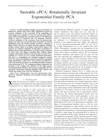
6074IEEE TRANSACTIONS ON IMAGE PROCESSING, VOL. 29, 2020Fig. 3. Eigenimages estimated from noisy XFEL data using PCA, steerable PCA (sPCA), ePCA, and steerable ePCA (sePCA), ordered by eigenvalues. Inputimages are corrupted by poisson noise with mean photon count 0.01 (shown in Figure 1b).which has a block diagonaland is decoupled for each structuremax(k) , withangular frequency, B kk kBmaxR k,qk,qf (r ) gc 1 (r ) gc 2 (r ) r dr.Bq(k) (23)1 ,q20The radial integral in Eq. (23) is numerically evaluated usingthe Gauss-Legendre quadrature rule [47, Chap. 4], whichdetermines the locations of nr 4c R points {r j }nj r 1 on theinterval [0, R] and the associated weights w(r j ). The integralin Eq. (23) is thus approximated bynr k,qk,qBq(k) f (r j ) gc 1 r j gc 2 r j r j w(r j ). (24)1 ,q2j 1The recoloring step is also decoupled for each angularfrequency sub-block. The heterogenized covariance estimatorsare (k)(k)She B (k) · Sh,η· B (k) .(25)γkSimilar to Eq. (23), we define D (k) which will be used to scalethe heterogenized covariance matrix estimator (see Eq. (27))and denoise the expansion coefficients (see Eqs. (29) and (30)), Dq(k)1 ,q2R0nr k,qk,qf (r ) gc 1 (r ) gc 2 (r ) r drk,qk,qf (r j ) gc 1 r j gc 2 r j r j w(r j ).(26)j 1In Alg. 1, Steps 11 and 12 summarize the recoloringprocedure.F. Scaling rk (k)(k)(k)The eigendecomposition of She gives She i 1 v̂ i v̂ i(k) . The empirical eigenvalues are tˆ v̂ (k) 2 which is abiased estimate of the true eigenvalues of the clean covariancematrix X . In [25, Sec. 4.2.3], a scaling rule was proposedto correct the bias. We extend it in Steps 13 and 14 in Alg. 1(k)by ato the steerable case and scale each eigenvalue of She(k)parameter α̂ , 1 ŝ 2 τ (k), for 1 ŝ 2 τ (k) 0 and ĉ2 0(k)2α̂ ĉ 0otherwise(27)where the parameter τ (k) ance matrices areSs(k)rk trD (k)pk· ˆ. v̂ (k) 2α̂i(k) v̂ i(k) v̂ i(k) The scaled covari.(28)i 1The rotationally invariant covariance kernel S((x, y), (x , y )) kmax(k)(k)iswellapproximatedbyk kmax G (x, y)Ss k,qG (k) (x , y ) , where G (k) contains IFT of all ψcwith angular frequency k (see Step 17) in Alg. 1). Thecomputational complexity of steerable ePCA is O(n L 3 L 4 ),same as steerable PCA, and it is lower than the complexityof ePCA which is O(min(n L 4 L 6 , n 2 L 2 n 3 )).In summary, Step 14 scales the heterogenized covariancematrix She . The covariance matrix in the original pixel domain(k)is efficiently computed from Ss in Step 17.Authorized licensed use limited to: University of Illinois. Downloaded on February 10,2021 at 16:51:56 UTC from IEEE Xplore. Restrictions apply.
ZHAO et al.: STEERABLE ePCA: ROTATIONALLY INVARIANT EXPONENTIAL FAMILY PCA6075Fig. 4. Error of covariance matrix estimation, measured as the (a) operator norm and (b) Frobenius norm of the difference between each covariance estimateand the true covariance matrix. The sample size n ranges from 100 to 140,000.Fig. 5. The estimated number of signal principal components using PCA,sPCA, ePCA and sePCA. Images are corrupted by poisson noise with meanper pixel photon count 0.01.Fig. 6. The runtime for computing the principal components using PCA,sPCA, ePCA and sePCA. Images are corrupted by poisson noise with meanper pixel photon count 0.01.G. DenoisingAs an application of steerable ePCA, we develop a methodto denoise the photon-limited images. Since the Fourier-Besselexpansion coefficients are computed from the prewhitenedimages, we first recolor the coefficients by multiplying B (k)with A(k) and then we apply Wiener-type filtering to denoisethe coefficients. For the steerable basis expansion coefficients A(k) with angular frequency k 0,Â(k) Ss(k) D (k) Ss(k) 1B (k) A(k) .(29)For k 0, we need to take into account the rotationallyinvariant mean expansion coefficients,Â(0) Ss(0) DD(0)(0) Ss(0) 1(0)i ,coefficients âk,qp00,qX̂ i (x, y) (0)B A 1D (0) Ss(0)Ā1 n.Fig. 7.Sample clean and noisy images of randomly rotated yale facedatabase B
estimator, constructed in a deterministic and non-iterative way using moment calculations and shrinkage.ePCA was shown to be more accurate than PCA and its alternatives for exponential families. It has computational cost similar to that of PCA, substantial theoretical justification building on random matrix theory, and interpretable output.