Transcription
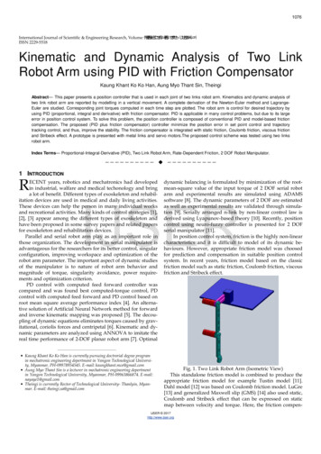
1076International Journal of Scientific & Engineering Research, Volume ȱŞǰȱ ȱŗŘǰȱ ȬŘŖŗŝISSN 2229-5518Kinematic and Dynamic Analysis of Two LinkRobot Arm using PID with Friction CompensatorKaung Khant Ko Ko Han, Aung Myo Thant Sin, TheingiAbstract— This paper presents a position controller that is used in each joint of two links robot arm. Kinematics and dynamic analysis oftwo link robot arm are reported by modelling in a vertical movement. A complete derivation of the Newton-Euler method and LagrangeEuler are studied. Corresponding joint torques computed in each time step are plotted. The robot arm is control for desired trajectory byusing PID (proportional, integral and derivative) with friction compensator. PID is applicable in many control problems, but due to its largeerror in position control system. To solve this problem, the position controller is composed of conventional PID and model-based frictioncompensation. The proposed (PID plus friction compensator) controller minimize the position error in set point control and trajectorytracking control, and thus, improve the stability. The friction compensator is integrated with static friction, Coulomb friction, viscous frictionand Stribeck effect. A prototype is presented with metal links and servo motors.The proposed control scheme was tested using two linksrobot arm.Index Terms— Proportional-Integral-Derivative (PID), Two Link Robot Arm, Rate-Dependent Friction, 2 DOF Robot Manipulator.—————————— ——————————1 INTRODUCTIONRECENT years, robotics and mechatronics had developedin industrial, walfare and medical techonology and bringa lot of benefit. Different types of exoskeleton and rehabilitation devices are used in medical and daily living activities.These devices can help the person in many individual worksand recreational activities. Many kinds of control strategies [1],[2], [3] appear among the different types of exoskeleton andhave been proposed in some survey papers and related papersfor exoskeleton and rehabilitation devices.Parallel and serial robot arm play as an important role inthose organization. The development in serial manipulator isadvantageous for the researchers for its better control, singularconfiguration, improving workspace and optimization of therobot arm parameter. The important aspect of dynamic studiesof the manipulator is to nature of robot arm behavior andmagnitude of torque, singularity avoidance, power requirements and optimization criterion.PD control with computed feed forward controller wascompared and was found best computed-torque control, PDcontrol with computed feed forward and PD control based onroot mean square average performance index [4]. An alternative solution of Artificial Neural Network method for forwardand inverse kinematic mapping was proposed [5]. The decoupling of dynamic equations eliminates torques caused by gravitational, coriolis forces and centripetal [6]. Kinematic and dynamic parameters are analyzed using ANNOVA to imitate thereal time performance of 2-DOF planar robot arm [7]. Optimaldynamic balancing is formulated by minimization of the rootmean-square value of the input torque of 2 DOF serial robotarm and experimental results are simulated using ADAMSsoftware [8]. The dynamic parameters of 2 DOF are estimatedas well as experimental results are validated through simulation [9]. Serially arranged n-link by non-linear control law isderived using Lyapunov-based theory [10]. Recently, positioncontrol using neuro-fuzzy controller is presented for 2 DOFserial manipulator [11].In position control system, friction is the highly non-linearcharacteristics and it is difficult to model of its dynamic behaviours. However, appropriate friction model was choosedfor prediction and compensation in suitable position controlsystem. In recent years, friction model based on the classicfriction model such as static friction, Coulomb friction, viscousfriction and Stribeck �——— Kaung Khant Ko Ko Han is currently pursuing doctrorial degree programin mechatronic engineering depertment in Yangon Technological University, Myanmar, PH-09978954545. E-mail: kaungkhant.mce@gmail.com Aung Myo Thant Sin is a lecturer in mechatronic engineering depertmentin Yangon Technological University, Myanmar, PH-09963866874. E-mail:nayaye1@gmail.com Theingi is currently Rector of Technological University- Thanlyin, Myanmar. E-mail: theingi.sa@gmail.comFig. 1. Two Link Robot Arm (Isometric View)This standalone friction model is combined to produce theappropriate friction model for example Tustin model [11].Dahl model [12] was based on Coulomb friction model. LuGre[13] and generalized Maxwell slip (GMS) [14] also used static,Coulomb and Stribeck effect that can be expressed on staticmap between velocity and torque. Here, the friction compen-IJSER 2017http://www.ijser.org
1077International Journal of Scientific & Engineering Research, Volume ȱŞǰȱ ȱŗŘǰȱ ȬŘŖŗŝISSN 2229-5518sation in proposed position controller was based on static,Coulomb, viscous models and Stribeck effect. From this staticmodel can conduct to LuGre and generalized Maxwell slip(GMS). Model based friction compensation can be used instimulation, gain tunning and stability analyse [16].This paper concerns the kinematic and dynamic analysis of2 link robot arm (see in Fig. 1) and PID controller with frictioncompensator. A two links robot arm’s kinematics, and dynamic equations are obtained and dynamic analysis is the derivingequations, the relationship between force and motion in a system. The Newton-Euler method and Lagrange are derivedcompletely. The corresponding joint torques computed in eachtime step are plotted and choosed the motor from aid of thisresult. The proposed (PID plus friction compensator) controller minimize the position error in set point control and trajectory tracking control, and thus, improve the stability. The friction compensator is integrated with static friction, Coulombfriction, viscous friction and Stribeck effect.This report is organized as follows. Section 2 discusses thekinematic and section 3 is dynamic analysis. Section 4 is proposed position controller and fricition compensator. Section 5is the experiemental results. Section 6 & 7 are the discussionand conclusion.Fig. 2. Two Link Robot Arm for Forward Kinematic.2.2 Inverse KinematicGiven the position and orientation of the end effector relative to the base frame compute all possible sets of joint anglesand link geometries which could be used to attain the givenposition and orientation of the end effector. The inverse kinematic transformation for the idealized two-joint robot armmodel (Fig. 3) can be represented mathematically:IJSERx 2 y 2 l12 cos 2 (θ1 ) l 22 cos 2 (θ1 θ 2 ) 2l1l 2 cos (θ1 ) cos (θ1 θ 2 ) 2 KINEMATIC OF TWO LINK ROBOT ARMl12 sin 2 (θ1 ) l 22 sin 2 (θ1 θ 2 ) 2l1l 2 sin (θ1 ) sin (θ1 θ 2 )Robot kinematics applies geometry to the investigationthe movement of multi-degree of freedom kinematic chainsthat form the structure of robot arm.2.1 Forward KinematicGiven the joint angles and the links geometry, computethe orientation of the end effector involved in the execution ofa movement is kinematic. A limb, as a mechanical device,converts muscle lengths and joint angles to hand positions.This process is referred to as forward kinematics. In Fig. 2, anidealized model of this transformation for movements in avertical plane is illustrated. The arm is modeled as two rigidlinks of length 260 mm and 230 mm, the links rotate abouthorizontal parallel axes that are fixed with respect to the links.For this idealized model the forward kinematics from jointangles (θ1 , θ 2 ) to hand position (x, y) are given by(1)x l1 cos (θ1 ) l2 cos (θ1 θ2 )(3)To control a two-joint robot arm, the inverse kinematictransformation could be implemented as a digital computerprogram as following:θ2 a tan 2( sin θ2 ,cos θ2 ) a tan 2( 1 cos 2 θ2 ,cos θ2 ) a tan 2( 1 (x 2 y 2 l12 l22 x 2 y 2 l12 l22),)2l1l22l1l2θ1 a tan 2(y,x) a tan 2(k 2 ,k1 )(4)(5)Wherek1 l1 l2 cosθ2(6)k 2 l 2 sin θ2(7)(2)y l1 sin (θ1 ) l2 sin (θ1 θ2 )Given a desired hand position, choose the appropriatemuscle lengths and corresponding joint angles to achieve thatposition. The transformation from desired hand position to thecorresponding joint angles and muscle lengths is known as theinverse kinematic transformation. Internal models of arm kinematics are also useful in choosing torques at the joints of thearm to achieve a particular force and torque between the handand some external object. Learning to move accurately mayinvolve building internal models of kinematic transformations.Fig. 3. Two Link Robot Arm for Inverse Kinematic.IJSER 2017http://www.ijser.org
1078International Journal of Scientific & Engineering Research, Volume ȱŞǰȱ ȱŗŘǰȱ ȬŘŖŗŝISSN 2229-55183 DYNAMIC OF TWO LINKS ROBOT ARMAs demonstrated in this document, the numbering for sectionsupper case Arabic numerals, then upper case Arabic numerals,separated by periods. Initial paragraphs after the section titleare not indented. Only the initial, introductory paragraph hasa drop cap.3.1 Lagrangian and Newton-Euler FormulationsIt is necessary to analyze the dynamic characteristics of amanipulator in order to control it, to simulate it, and to evaluate its performance. A manipulator is most often an open-looplink mechanism, which may not be a good structure from theviewpoint of dynamics (it is usually not very rigid, its positioning accuracy is poor, and there is dynamic couplingamong its joint motions). This structure, however, allows us toderive a set of simple, easily understandable equations of motion.Two methods for obtaining the equations of motion arewell known: the Lagrangian and the Newton-Euler formulations. At first the Lagrangian formulation was adopted. Thisapproach has a drawback in that the derivation procedure isnot easy to understand physically; it uses the concept of theLagrangian, which is related to kinetic energy. However, theresulting equation of motion is in a simple, easily understandable form and is suitable for examining the effects of variousparameters on the motion of the manipulator.Recently, as the need for more rapid and accurate operation of manipulators has increased, the need for real-timecomputation of the dynamics equations has been felt morestrongly. The Newton-Euler formulation has been found to besuperior to the Lagrangian formulation for the purpose of fastcalculation. Also, the Newton-Euler formulation is valid forcomputed torque control.The following Fig. 5 is the front view of the experimentalsetup of the two link robot arm is drawing using the SolidWrok. The dimensions of the two link robot arm is expressedin following Table 1;TABLE 1DIMENSION OF THE 2-LINKS ROBOT ARMParts of the Robot ArmDimension of the PartsLink -1 (Length x Width(260 x 30 x 10) mmx Thickness)Link -2 (Length x Width(230 x 30 x 10) mmx Thickness)Diameter of Motor 1 and38 mm2Shaft Diameter of Motor6 mm1 and 2Base Plate (Length x(250 x 200 x 10) mmWidth x Thickness)IJSER3.2 Lagrangian FormulationWe will derive the dynamics equation of a two-link robotarm movement. Let us consider the robot arm in Fig. 4. Thefollowing notations are used in the figure:θ i the joint angle of joint-i,mi the mass of link-i, I i the moment of inertia of link-i about the axis that passesthrough the center of mass and is parallel to the Z-axis, andli the length of link-iFig. 5. Drawing for Two Link Robot Arm (Front View)We assume that the first joint driving torque τ 1 acts between the base and link - 1, and the second joint drivingtorque τ 2 acts between links 1 and 2.Choosing q1 θ1 and q2 θ 2 as generalized coordinates,we will find the Lagrangian function. Let the kinetic energyand the potential energy for link - i be K i and Pi respectively.For link - 1, we have11 222(8)K1 m1 l g1 θ&1 I 1 θ&1 ,22(9)P1 m1 gˆ l g 1 S1,where ĝ is the magnitude of gravitational acceleration. Forlink - 2, since the position of its center of mass s2 [ s2 x , s2 y ]T isgiven by(10)s2 x l1 C1 l g 2 C12 ,s2 y l1 S1 l g 2 S12 ,Fig. 4. Dynamic Analysis of Two Link Robot Arm.We have the relationT22s& s& l θ& l2IJSER 2017http://www.ijser.org2112g22(θ&1 θ&2 )2 2l1l g 2 C 2(θ&1 θ&1 θ&2 ).(11)(12)
1079International Journal of Scientific & Engineering Research, Volume ȱŞǰȱ ȱŗŘǰȱ ȬŘŖŗŝISSN 2229-5518Also,30 degree and q(2) 30 60 degree11 TK 2 m2 s&2 s&2 I 2(θ&1 θ&2 )222(13)P2 m2 gˆ (l1S1 l g 2 S12 ).(14)andCalculating L K1 K2 - Pl - P2 and the equations of motion for the two-link arm are: 222τ1 [m1l g1 I1 m2(l1 l g 2 2l1l g 2 C 2 ) I 2 ]θ&&1 [m2(l g 2 2 l1l g 2 C 2 ) I 2 ]θ&&2 m2 l1l g 2 S 2( 2θ&1θ&2 θ&2 2 ) (15) m1 gˆ l g1C1 m2 gˆ(l1C1 l g 2 C12 ), 22τ [m2(l g 2 l1l g 2C 2 ) I 2 ]θ&&1 (m2 l g 2 I 2 )θ&&2 m2l1l g 2 S 2 θ&1 m2 gˆ l g 2 C12 .2This can also be rewritten as2τ1 M 11θ&&1 M 12θ&&2 h12 2θ&2 2h112θ&1θ&2 g1,2τ 2 M 21θ&&1 M 22θ&&2 h211θ&1 g 2 ,Where, 222M 11 m1l g1 I1 m2(l1 l g 2 2l1l g 2 C2 ) I 2 , 2M 12 M 21 m 2 (l g 2 l1 l g 2 C2 ) I 2 , 2M 22 m2 l g 2 I 2 ,(16)(17)Fig. 7. Dynamic Analysis of 2-Links Robot Arm, q(1) 0 90degree and q(2) 90 180 degree(18)(19)IJSER(20)(21)h12 2 h112 h211 m2 l1 l g 2 S 2 ,(22)g1 m1 gˆ l g1 C1 m2 gˆ (l1 C1 l g 2 C12 ),(23)g 2 m2 gˆ l g 2 C12.(24)Inverse dynamic analysis has been done for the joint spacespiral trajectory considered for the controller design. Fig. 6,Fig. 7, Fig. 8 illustrate the driving torques (τ1, τ2) of the 2 linkmanipulator from the knowledge of the trajectory equation interms of time. The following simulation result is based on Lagrange Formulation.In Fig. 6, dynamic analysis of 2 links robot arm and q(1)(Joint 1 angle) is setting 0 to 30 degree and q(2) is setting 30 to60 degree. The initial torque for joint - 1 is near 1.4 N-m andjoint – 2 is about -0.225 N-m.In Fig. 7, dynamic analysis of 2 links robot arm and q(1)(Joint 1 angle) is setting 0 to 90 degree and q(2) is setting 90 to180 degree. The initial torque for joint - 1 is near 1.4 N-m andjoint – 2 is about -0.225 N-m.Fig. 8. Dynamic Analysis of Two Link Robot Arm, q(1) 0 90 degree and q(2) 90 360 degreeIn Fig. 8, dynamic analysis of 2 links robot arm and q(1)(Joint 1 angle) is setting 0 to 90 degree and q(2) is setting 90 to360 degree. The initial torque for joint - 1 is near 1.4 N-m andjoint – 2 is about 0.22 N-m.Therefore, the maximum torque of pololu motor is 1.5 Nm is enabled, the above three Fig. 6, Fig. 7, Fig. 8 have maximum torque usage is around 1.55 N-m and 1.6 N-m. This motor selection is suitable for trajectory tracking control system.3.3 Newton-Euler FormulationIn order to illustrate the use of the N-E equations of motion, the same two-link robot arm with revolute joints asshown in Fig. 4.All the rotation axes at the joints are along the z-axis perpendicular to the paper surface. The physical dimensions, center of mass, and mass of each link and coordinate systems aregiven in Table 1.First, we obtain the rotation matrices from Fig. 4: C1R1 S1 0 C10R1 S1 00Fig. 6. Dynamic Analysis of Two Links Robot Arm, q(1) 0 IJSER 2017http://www.ijser.org S1 0 C 2 S 2 0 C12 S12 0 (25)C1 0 1R2 S 2 C 2 0 0R2 S12 C12 0 0 00 1 01 01 S1 0 C 2 S 2 0 C12 S12 0 (26)C1 0 1R2 S 2 C 2 0 0R2 S12 C12 0 0 00 1 0 1 0 1
1080International Journal of Scientific & Engineering Research, Volume ȱŞǰȱ ȱŗŘǰȱ ȬŘŖŗŝISSN 2229-5518We assume the following initial conditions: ω0 ω& 0 v0 0and v&0 ( 0, g , 0)T with g 9.8062 m/s2.Forward equations for i 1, 2. Compute the angular velocityfor revolute joint for i 1, 2.Therefore, for i 1, with ω0 0 , we have:1R0 ω1 1R0(ω0 z 0θ&1 ) C1 S1 0 S1 C1 0 00 1 For i 2, we have:2R0 ω2 2R1( 1R0 ω1 z0 θ&2 ) 0 0 0 θ& 0 θ& 1 1 1 1 (27) C 2 S 2 0 0 0 0 (28) & & & & S 2 C 2 0 0 θ1 0 θ2 0 (θ1 θ2 ) 0 1 1 0 1 1 Compute the angular acceleration for revolute joints for i 1, 2.For i 1, with ω& 0 ω0 0 , we have:1R ω& 1R (ω& z θ&& ω z θ& ) ( 0 ,0 ,1 )T θ&&(29)01000 100 11For i 2, we have:2 1 1 2 C1 C1 1 C1 S1 0 2 1 21s1 S1 1R0 s1 S1 C1 0 S1 0 2 2 00 1 0 0 0 Thus, 1 1 2 0 2 0 0 2 lθ&1 gS1 && &&1R0 a1 0 θ1 0 0 0 0 lθ1 gC1 1 0 θ&1 θ&1 0 0 1 &2 2 θ1 gS1 1 θ&&1 gC1 2 0 For i 2, we have:2R0 a2 ( 2R0 ω& 2 ) ( 2R0 s2 ) ( 2R0 ω2 ) [( 2R0 ω2 ) ( 2R0 s 2 )] 2R0 v&2 (34)Where 1 2 C12 C12 1 s 2 S12 2R0 s 2 S12 2 0 0 R0 ω& 2 2R1( 1R0 ω& 1 z 0 θ&&2 ( 1R0 ω1 ) z 0 θ&2 ) ( 0 ,0 ,1 )T (θ&&1 θ&&2 ) (30)IJSERCompute the linear acceleration for revolute joints for i 1, 2.For i 1, with v&0 (0, g , 0) T , we have:1R0 v&1 ( 1R0 ω& 1 ) ( 1R0 P1 ) ( 1R0 ω1 ) [( 1R0 ω1 ) ( 1R0 P1 )] 1R0 v&0 (31) 0 0 0 0 0 gS1 && & & 0 θ1 0 0 θ1 0 θ1 0 gC1 1 1 1 1 1 0 2& lθ1 gS1 lθ&&1 gC1 0 R0 v&2 ( 2R0 ω& 2 ) ( 2R0 P2 ) ( 2R0 ω2 ) [( 2R0 ω2 ) ( 2R0 P2 )] 2R1( 1R0 v&0 ) 1 1 0 0 0 22 2R0 a2 0 0 0 0 0 θ&&1 θ&&2 0 θ&1 θ&2 θ&1 θ&2 0 l(S 2 θ&&1 C 2 θ&12 θ&12 θ&12 2θ&1θ&2 ) gS12 l(θ&&1 θ&&2 C 2θ&&1 S 2θ&&2 ) gC12 0 (32) 0 1 0 0 1 0 0 0 0 0 θ&&1 θ&&2 0 θ&1 θ&2 θ&1 θ&2 0 2& C2 S 2 0 lθ1 gS1 S 2 C2 0 lθ&&1 gC1 00 1 0 l(S 2θ&&2 C 2θ&12 θ&12 θ&22 2θ&1θ&2 ) gS12 l(θ&&1 θ&&2 C 2 θ&&1 S 2θ&12 ) gC12 0 Compute the linear acceleration at the center of mass for links1 and 2:For i 1, we have:1 1 C12 1 0 2 2 1 0 S12 0 2 1 0 0 Thus,For i 2, we have:2S12C120R0 a1 ( 1R0 ω& 1 ) ( 1R0 s1 ) ( 1R0 ω1 ) [( 1R0 ω1 ) ( 1R0 s1 )] 1R0 v&1 (33) &&&2 1 &2 1 &2 & & l(S 2θ1 C2 θ1 2 θ1 2 θ 2 θ1θ2 ) gS12 11 l(C 2θ&&1 S 2 θ&12 θ&&1 θ&&2 gC12 ) 22 0 Backward equations for i 2, 1. Assuming no-load conditions, f 3 n3 0 . We compute the force exerted on link - i for i 2, 1.For i 2, with f 3 0 , we have:2(35)R0 f 2 2R3( 3R0 f 3 ) 2R0 F2 2R0 F2 m2 2 R0 a2 &&&2 1 &2 1 &2 & & m2 l(S 2 θ1 C2 θ1 2 θ1 2 θ 2 θ1θ 2 ) gm2 S12 11 m2 l(C2 θ&&1 S 2 θ&12 θ&&1 θ&&2 ) gm2 C12 22 0 For i 1, we have:1R0 f1 1R2( 2R0 f 2 ) 1R0 F1WhereIJSER 2017http://www.ijser.org(36)
1081International Journal of Scientific & Engineering Research, Volume ȱŞǰȱ ȱŗŘǰȱ ȬŘŖŗŝISSN 2229-551811 m2 l(S 2 θ&&1 C 2 θ&2 θ&12 θ&22 θ&1θ&2 ) gm2 S12 220 110 m2 l(C 2 θ&&1 S 2 θ&12 θ&&1 θ&&2 ) gm2 C12 m1 1 R0 a122 1 0 S2 C 2 S 2 0C20 &2 1&2 &2& & 1&& && m2 l[ θ1 2 C 2(θ1 θ 2 ) C 2 θ1θ 2 2 S 2(θ1 θ 2 )] m g(C S C S ) 1 m lθ& 2 m gS 21222121111 2 1122&&&&&&&&&& m2 l[θ1 S 2(θ1 θ 2 ) S 2 θ1θ 2 C 2(θ1 θ 2 )] 22 1&& m gC mgC mlθ 211 111 2 0 R0 n2 ( 2R0 p2 2R0 s2 ) ( 2R0 F2 ) 2R0 N 2 4(37)Wherep2 lC12 C12 lS12 2R0 p 2 S12 0 0Thus,S120 0 1 0 1m2 l 2 12 0(40)FRICTION IDENTIFICATIONMostly, position control system based on the conventionalProportional-Integral-Derivative (PID) method. The conventional Proportional-Integral-Derivative (PID) equation is asfollowed:u PID Ke(t) L e(t)dt B lC12 l lS12 0 0 0 de(t)dt(41)Where uPID is the controller output from the controller and K, Land B are positive real numbers, which represent the proportional, integral and derivative gains. The e(t) is define as p(t)(actual position) that is subtracted from pd(t) (desired position).1 2 1 2 2 1 m2 l(S 2 θ&&1 C 2 θ&1 θ&1 θ&2 θ&1θ&2 ) gm2 S12 22 2 112R0 n2 0 m2 l(C 2 θ&&1 S 2 θ&12 θ&&1 θ&&2 ) gm2 C12 22 0 0 00 1 0m2 l 2 12 00 141m1l 2 θ&&1 m2 l 2 θ&&1 m2 l 2 θ&&2 m2 C 2l 2θ&&1333112 m2l C 2θ&&2 m2 S 2l 2 θ&1θ&2 m2 S 2 l 2θ&222211 m1 glC1 m2 glC12 m2 glC122IJSERC120(39)111 m2 l 2 θ&&1 m2 l 2 θ&&2 m2 l 2 C 2 θ&&133211 m2 glC12 m2 l 2 S 2 θ&1222For i 1, with b1 0 , we have:τ1 ( 1R0 n1 )T ( 1R0 z 0 )Compute the moment exerted on link - i for i 2, 1.For i 2, with n3 0 . we have:2τ 2 ( 2R0 n2 )T ( 2R1 z 0 )4.1 Rate Depended Friction IdentificationFor the friction compensation, it is required Polou DC motor with two channels linear quadrature encoder and 100:1gear transmission, arm at the motor sharft and basement forfixing the motor in it. Motor is driven by L298N driver with12V DC.For the control algorithm, it is used LPC 1768, ARM basedCortex-M3 microcontroller, the clock frequency is 96 MHz.The ARM microcontroller has many timers and serial connectors. Personal computer (PC) is used for serial monitoring andprogramming for microcontroller. 0 0 θ&&1 θ&&2 0 0 1 1112 &&2 &&22&&& m2 l θ1 m2 l θ 2 m2 l (C 2 θ1 S 2 θ1 ) m2 glC12 322 3 For i 1, we have:1R0 n1 1R2 [ 2R0 n2 ( 2R0 p1 ) ( 2R0 f 2 )] ( 1R0 p1 1R0 s1 ) ( 1R0 F1 ) ( 1R0 N1 )(38)Wherep1 lC1 lC 2 l 2 1 lS1 R0 p1 lS 2 R0 p1 0 0 0 0 Thus,1R0 n1 1R2( 1R0 n2 ) 1R2 [( 2R0 p1 ) ( 2R0 f 2 )]1,0 ,0 ] T ( 1R0 F1 ) ( 1R0 N1 )2Finally, we obtain the joint torques applied to each of the jointactuators for both links.For i 2, with b2 0 , we have: [Fig. 9. Position Control Block Diagram for Friction IdentifitionExperimentFriction model allows different parameter sets for positiveand negative velocity regime and easily identifiable parameters. The model clearly separates the high and low velocityregime. It can easily be implemented and introduced in realtime control algorithms. This experiment (see Fig. 9) is findingthe parameters that actually appear from the friction force(passive) in gear box of the motor and friction in motor (electro-mechanical device has friction).IJSER 2017http://www.ijser.org
1082International Journal of Scientific & Engineering Research, Volume ȱŞǰȱ ȱŗŘǰȱ ȬŘŖŗŝISSN 2229-5518gain and perform stimulation.This paper presents an encoder-based friction compensator for a geared actuator. The compensator only requires theencoder signal as its input to enhance the system.Most of existing friction compensation techniques arebased on friction models that uses the velocity as its input. Itcan be seen in Fig. 13. The friction can be found at low velocitythat is from derivative of the position of the encoder. In thissaturation, the system meets with static friction state, beingsensitive to external force. When the velocity is more andmore, the compensator produces a force to cancel the frictionforce based on a predefined rate at friction model.TABLE 2PARAMETER VALUES OBTAINED FROM FIG. 11Fig. 10. Torque and Velocity Curve to identify the frictionforceThis Curve is Torque and Velocity Curve to identify the friction force as shown in Fig. 10. Because Friction is a Function ofVelocity.When the motor is feed sinusoidal input in Fig. 9, the motor genate speed and torque and that is put on the coordinatesystem in Fig. 10. The data from Fig. 10 is divided by two andthis data is stored in Matlab software. After that Fig. 11 is generated from this storage data.According to the Fig. 11, static friction Fs can be seen invertical positive and negative peak point of red line. Fs isgreater than the other frictions magnitude. Static friction isalso depending on the velocity that is at zero condition, at thattime static friction force appears.Parameter Fs Fc Fv vs Fs- FcFvvsUnitN-m N-m N-m deg/s N-m N-m N-m deg/sValue39 24.61 1 1.765 38 23.89 1.326 1.82The proposed friction model is as followed:F f ( Fc ( Fs Fc )eIJSER v vs) sign(v ) Fv v(42)Where Fs, Fc, Fv, is the Static, Coulomb, Viscous friction and vsis the Stribeck velocity. δ is an additional empirical parameter.v is the velocity estimated from encoder. Table 2 parametervalues in friction model eq. (42).5EXPERIMENTAL RESULTThis section presents the results of experiments showingthe effectiveness of the proposed PID and PID with frictioncontrol scheme are illustrated by using a two link robot(2DOF) positioning system. The performance of the proposedcontroller is compared with a PID with friction compensator.For this experiment, it is required two sets of Polou DC motorwith two channels linear quadrature encoder and 100:1 geartransmission. Motor is driven by L298N driver with 12V DC.For the control algorithm, it is used NXP LPC 1768, the clockfrequency is 96 MHz. The microcontroller is connected to a PCcomputer through USB cable. The PC is used for data monitoring and acquisition by Cool Term Serial Data Logger. The encoder resolution is 65.33 pulses per revolution and entire resolution of the motor shaft is 6533 pulses per revolution.Fig. 11. This Curve is the Rate-Depended Friction Identification Curve. Friction Parameter is Received from this Curve.4.1 Modeling of Friction CompensatorFriction is the important part for control system in highquality precision mechanisms, electro-mechanical devices,hydraulic and pneumatic system. Due to the effect of friction,the control system does not reach the desired position, to solvethis problem, the control engineer used higher gain controlloops, that is not better choice, inherently require a suitablefriction model to compensate and still in precise position. Agood model is also required to analyse stability, find controllerIJSER 2017http://www.ijser.orgFig. 12. Experimental Setup of the 2-Links Robot Arm
1083International Journal of Scientific & Engineering Research, Volume ȱŞǰȱ ȱŗŘǰȱ ȬŘŖŗŝISSN 2229-55185.1 Proposed Position ControllerThe proposed position controller is the combination of theconvential PID controller with friction compensator. The controller block diagram is expressed in Fig. 13.Fig. 13. Proposed Position Controller Block Diagram5.1 Set Point and Trajectory Tracking Control with PIDTo validate the proposed framework, following experimental steps were passed through step by step. The first step ofexperiment is PID gain turning for Joint – 1. To do this gainturning, we had to set desired input (blue line) by step or setpoint input (this is shown in Fig. 14 and Fig. 15) in followingblock diagram. Gain turning was trial and error method. Trialand error method is easy.duced the torque command that was equal to the product ofKp and error value. In this condition, the Kp gain was increaseto reach the appropriate torque, however, Kp turning wasstopped when the actual angle beyond the desired angle. Thecondition beyond the desired angle was called overshoot region. This overshoot effect was recovered by the derivativegain Kd, was turned to reduce the actual angle to reach thedesired angle, however, the actual angle decreased under theactual angle which was called undershoot. To compensate theundershoot effect, the Ki was turned to reach desired angle.Integral turning, absolutely based on sampling interval. Although, integral term did not recover the steady-state region.Friction compensator was used together with PID controllerand it could recover steady-state error even when the sampling frequency is low. PID Gain value is seen in Table 3.TABLE 3Parameter of PID ControllerPID ParemeterGainKp10Ki0.05Kd0.05IJSERFig. 14. PID Set Point Control Result of Joint 1 of 2-Links RobotArmFig. 15. PID Set Point Control Result in Joint 2 of 2-Links RobotArmThe first experiment was the gain turning for Joint – 1 PIDcontroller in Fig. 14. Here, desired input was setting up at 60degree, the controller had error input at this condition becauseactual angle is less than desired angle. The controller pro-Fig. 16. PID Trajectory Tracking Control Result in Joint 1 of 2Links Robot ArmFig. 17. PID Trajectory Tracking Control Result in Joint 2 of 2Links Robot ArmIn Fig. 14, the maximum joint torque was produced inIJSER 2017http://www.ijser.org
1084International Journal of Scientific & Engineering Research, Volume ȱŞǰȱ ȱŗŘǰȱ ȬŘŖŗŝISSN 2229-5518transient region, PWM is 100 percent ON [255 units i.e. Arduino PWM value]. At this transient region, PID must beovershoot but it reached near the desired angle. Joint 1 did notreach the desired angle in steady state region.In Fig. 15, the maximum joint torque was produced intransient region, PWM is almost 100 percent ON [255 units i.e.Arduino PWM value.] At this transient region, PID had overshoot. Derivative term reduced the overshoot but it caused theundershoot. Joint 2 reached near desired angle in steady stateregion but integral term did not fully recover in steady stateregion. Therefore, friction compensation for joint 1 and 2 wereshown in Fig. 18 and Fig. 19.5.2 Set Point and Trajectory Tracing Control with PID Friction CompensatorFig. 16. and Fig. 18 PID trajectory tracking control result andPID with friction compensator result in joint 1 of robot arm didnot follow the desired trajectory. To answer this question, inversedynamic analysis of 2 links robot arm results is shown in Fig. 6,Fig. 7 and Fig. 8.6 DISCUSSIONForward kinematic and Inverse Kinematic are interned toAdmittance type force controller and dynamic and inversedynamic are formulated by the Newton
This paper concerns the kinematic and dynamic analysis of 2 link robot arm (see in Fig. 1) and PID controller with friction compensator. A two links robot arm's kinematics, and dynam-ic equations are obtained and dynamic analysis is the deriving equations, the relationship between force and motion in a sys-tem.