Transcription
Compositional Mining ofMulti-relational Biological DatasetsYing Jin, T. M. Murali, and Naren RamakrishnanDepartment of Computer Science, Virginia Tech, VA 24061, USAEmail: ut biological screens are yielding ever-growing streams of information about multipleaspects of cellular activity. As more and more categories of datasets come online, there is a correspondingmultitude of ways in which inferences can be chained across them, motivating the need for compositionaldata mining algorithms. In this paper, we argue that such compositional data mining can be effectivelyrealized by functionally cascading redescription mining and biclustering algorithms as primitives. Boththese primitives mirror shifts of vocabulary that can be composed in arbitrary ways to create rich chainsof inferences. Given a relational database and its schema, we show how the schema can be automaticallycompiled into a compositional data mining program, and how different domains in the schema can berelated through logical sequences of biclustering and redescription invocations. This feature allows usto rapidly prototype new data mining applications, yielding greater understanding of scientific datasets.We describe two applications of compositional data mining: (i) matching terms across categories of theGene Ontology and (ii) understanding the molecular mechanisms underlying stress response in humancells.Categories and Subject Descriptors: H.2.8 [Database Management]: Database Applications - Data Mining; I.2.6 [Artificial Intelligence]: LearningGeneral Terms: Algorithms.Keywords: compositional data mining, biclustering, redescription mining, bioinformatics, inductive logicprogramming.1
1IntroductionOur ability to interrogate the cell and computationally assimilate its answers is improving at a dramaticpace. For instance, the study of even a focused aspect of cellular activity, such as gene action, now benefitsfrom multiple high-throughput data acquisition technologies such as microarrays [7], genome-wide deletionscreens [13], and RNAi assays [25, 33, 34]. As more and more categories of biological data become online,there is a corresponding multitude of ways in which inferences can be chained across them, making it infeasible to prototype software for every conceivable analysis methodology. Different biologists have differentneeds and perspectives, and it is difficult to anticipate all the ways in which computational pipelines can beorganized.Consider the following two scenarios from bioinformatics applications. In the first, Scientist A desiresto identify a small set of C. elegans genes (perhaps encoding transcription factors) to knock-down (viaRNAi) in order to confer improved desiccation tolerance in the nematode. Scientist A might begin byidentifying those genes whose knock-down produces phenotypes related to improved desiccation toleranceand then find one or more transcription factors that combinatorially control the expression of these genes.In the second scenario, Scientist B is interested in analyzing similarities across gene expression programsunderlying aging in C. elegans and D. melanogaster. Scientist B might use DNA microarrays to measuregene expression across a wide time span in aging worms and flies; analyze these datasets individually tofind clusters of genes that are co-expressed under a subset of the time points; and determine if genes in aC. elegans cluster have a significant number of orthologs in a D. melanogaster cluster. To support sucharbitrary lines of reasoning, we need novel software tools that allow biologists to uniformly decomposecomplex analytical functions in terms of primitives that reason about and relate entities across biologicaldomains.We argue for compositional data mining (CDM) that, as the name indicates, is a way to construct complex data mining functions from simpler data mining primitives. Key to this idea is focusing on smallset of primitives that are powerful algorithms in their own right but which can be functionally cascadedin arbitrary ways. We present a software system (Proteus) that embodies the CDM concept using two suchprimitives—redescriptions and biclusters. These primitives serve complementary purposes and mirror shiftsof vocabulary that often accompany logical chains of reasoning (e.g., transcription factors regulated genes knock-down phenotypes for the desiccation scenario; worm age C. elegans genes D. melanogasterorthologs fly age in the aging scenario.) In our prior work [37, 40, 41, 44, 56], we have applied theseprimitives, individually, to gain significant insight into massive datasets. Using CDM, we combine theirexpressiveness to form chains of reasoning across domains.The rest of this paper is organized as follows. Section 2 uses examples to introduce the basic conceptsunderlying compositional data mining. Section 3 develops formalisms that capture the various elements ofCDM. Section 4 presents various algorithms that together help mine compositional patterns. Experimentalresults are presented next, first showcasing the effectiveness of our algorithms and optimizations in Section 5, followed by, in Section 6, examples of knowledge discovered from two application case studies:matching terms across categories of the gene ontology (GO) and understanding the molecular mechanismsunderlying stress response in human cells. Related research and conclusions are presented finally, in Sections 7 and 8.2
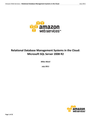
ntina RussiaChinaFranceUK USAANDRussiaChinaCubaFigure 1: (left) Example input to redescription mining. (right) Sample redescription. The expression B Y can be10 35 5 F0 6 F0 7 F5Ra FiCl nyoWi udynDa d yl 5ig MPht H h 75 6 F0Da FyCl ligo hRa udy t i10 5 nyh0Wi Fnd 5MPHredescribed into G re 2: (left) Example input to biclustering. (right) Layout of computed biclusters.2Compositional Data MiningCompositional data mining is not intended to be a one-size-fits-all data mining technique; rather, it is a wayof problem decomposition based on the notions of biclusters and redescriptions. We begin by reviewingthese primitives: whereas redescriptions relate object sets within a domain, biclusters relate object setsacross domains.2.1Redescription MiningAs the term indicates, to redescribe something is to describe anew or to express the same concept in adifferent way. The input to redescription mining is a set of objects and a collection of subsets defined overthis set. It is easiest to illustrate redescription mining using an everyday example. Consider the set of tencountries shown in Figure 1 and its four subsets, each of which denotes a meaningful grouping of countriesaccording to some intensional definition. For instance, the colors (G) green, (R) red, (B) blue, and (Y) yellow(from right, counterclockwise) refer to the sets ‘permanent members of the UN security council,’ ‘countrieswith a history of communism,’ ‘countries with land area 3, 000, 000 square miles,’ and ‘popular touristdestinations in the Americas (North and South).’ We will refer to such sets as descriptors. A redescription isa shift of vocabulary and the goal of redescription mining is to identify subsets that can be defined in at leasttwo ways using the given descriptors. An example redescription for this dataset is ‘Countries with land area 3, 000, 000 square miles outside of the Americas’ are the same as ‘Permanent members of the UN securitycouncil who have a history of communism.’ This redescription defines the set {Russia, China}, first by a set3
re 3: Finding transcription factors (TFs) whose knock-down induces improved desiccation tolerance in C. elegans. (left) Two biclusters (shaded rectangles) joined at the gene interface using an (approximate) redescription. (right)Compositional data mining schema, displaying the sequence of primitives. Here, arrows indicate redescriptions, anddotted lines indicate biclusters.Fly AgeGenesGenesWorm OrthologsFigure 4: Finding shared gene expression programs in adult aging in C. elegans and D. melanogaster. (left) Threebiclusters with redescription mining at the two gene interfaces. (right) Compositional data mining schema, displayingthe sequence of primitives. As before, arrows indicate redescriptions, and dotted lines indicate biclusterings.intersection of political indicators (G R), and second by a set difference involving geographical descriptors(B Y ). Notice that neither the set of objects to be redescribed nor the ways in which descriptor expressionsshould be constructed is input to the algorithm. The underlying premise of redescription analysis is that setsthat can indeed be defined in (at least) two ways are likely to exhibit concerted behavior and are, hence,interesting.2.2BiclusteringThe input to bicluster mining [32] is a set of instances of a relationship between two or more domains.Figure 2 describes relationships between dates (rows) and weather conditions (columns) in Blacksburg, VA.A bicluster is a subset of rows along with a subset of columns with the property that each row element isrelated to each column element (later we will utilize stricter notions of biclusters, but this definition willsuffice for this example). Figure 2 (bottom) lays out the seven biclusters in the matrix as contiguous submatrices by re-ordering the rows and columns of the matrix [24], repeating rows and columns if necessary.For example, the bicluster spanning rows three through six and columns two through four states that each ofthe four days from July 1–4, 2004 experienced each of the weather conditions “ 60 F,” “Daylight 10 h,”and “Cloudy.”2.3Composing Biclusters and RedescriptionsBoth redescriptions and biclusters have direct applications in bioinformatics. Redescriptions are useful inrelating gene sets from vocabularies based on cellular location (e.g., ‘genes localized in the mitochondrion’),transcriptional activity (e.g., ‘genes up-regulated two-fold or more in heat stress’), protein function (e.g.,‘genes encoding proteins that form the Immunoglobin complex’), or biological pathway involvement (e.g.,‘genes involved in glucose biosynthesis’). Similarly, biclusters are useful when we want to identify, e.g.,sets of genes together with sets of experiments or sets of phenotypes that exhibit concerted co-occurrences.However, they have complementary advantages and limitations.4
Redescriptions not only identify concerted sets but can also give meaningful characterizations of themin terms of data descriptors. This capability is akin to conceptual clustering [21, 35], where clusters arerequired to satisfy describability constraints. On the other hand, biclusters extensionally enumerate elementsof subsets from both domains; we must do a post-analysis of the contents of these sets to describe them.Conversely, redescription mining requires that all descriptors be stated over a common universal set, so thatdata spanning multiple relations must be collapsed into one of the underlying domains. For instance, arelationship between genes and transcription factors might be used to define descriptors over genes. On theother hand, biclustering retains the relational nature of information and models patterns in relations. It ishence natural to combine their complementary capabilities.To illustrate CDM, let us revisit the two scenarios from the introduction. The first scenario can be modeled by mining biclusters between genes and the transcription factors that regulate them, mining biclustersbetween genes and the phenotypes that result when they are knocked down, and connecting one side of thefirst bicluster to one side of the second bicluster using a redescription (see Figure 3). The second scenariocan be modeled by mining three biclusters—for the relationship between worm genes and worm age, for therelationship between fly genes and fly age, and for the orthology relationship between fly genes and wormgenes (see Figure 4). To cascade these three biclusters together, we can use two redescriptions as intermediaries, one redescribing worm genes, and the other redescribing fly genes. We can think of such cascadingas either the biclustering algorithm supplying descriptors to the redescription algorithm, or the redescriptionalgorithm specifying the objects that must participate in the biclustering. The results of such compositionscan be read sequentially from one end to the other, not unlike a story. For instance, for the first scenarioabove, we might find that ‘genes regulated by superoxide dismutase and catalase transcription factors, whenknocked down, will result in cells with a phenotype of hypersensitivity to oxidative stress.’ In general, suchcompositions can induce a graph of arbitrary topology in the underlying data model, as we will see later.Unlike the example in Figure 1, observe that both the CDM scenarios from Figs. 3 and 4 do not involveany constructive induction of descriptors in the redescriptions. There are situations where this feature isimportant, e.g., we may desire to find patterns such as “genes regulated by superoxide dismutase and catalasetranscription factors but not by transcription factors that control the cell cycle, when knocked down, willresult in cells with a phenotype of hypersensitivity to oxidative stress as well as abnormal cell size.” Tomine such patterns, each redescription must potentially relate two or more biclusters on either side. Inthis first paper on CDM, we define descriptors as the “projections” of biclusters onto the relevant domainsand focus on redescriptions with only one bicluster on each side, rather than on connecting set-theoreticcombination of bicluster projections.The Proteus vision of a CDM system is that a biologist can merely specify the domains that must participate in the composition (e.g., “TFs” and “phenotypes”) and the system automatically identifies a suitablecomposition of mining algorithms to relate the given domains. Observe that it can be infeasible to realize CDM by propositionalization, i.e., by first ‘multiplying’ out the original multi-relational dataset into asingle-relation dataset, mining patterns in the integrated set, and then unpacking the pattern to relate thegiven domains. Although propositionalization has proved to be viable in traditional inductive logic programming [29], such algorithms only need to relate individual objects across domains, whereas we mustrelate sets across domains, which are much larger in number and not defined a priori. In essence, CDM isrelational knowledge discovery [20] over sets, instead of objects. It is also wasteful to organize independent redescription and biclustering results across the different domains and relationships, since many of thepatterns mined would not participate in any connections.Another approach to CDM might be to start by computing biclusters in one relationship and use themto constrain the mining [8] of biclusters in a neighboring relationship. However, such constraint-based5
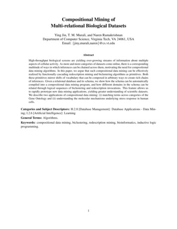
mining is ill-equipped to deal with the arbitrary expansion and contraction of descriptor sizes that CDMmust support. Nevertheless, there are several significant structural properties of CDM patterns that we willexploit to design efficient mining algorithms.The key contributions of this paper are as follows:1. We formulate the notion of compositional data mining as an approach to better conceptualize structured data mining problems. Rather than developing special purpose algorithms for every new type ofdataset or analysis goal, CDM helps to organize knowledge discovery tasks in a modular manner.2. Since CDM patterns connect sets of entities through alternating biclusters and redescriptions, wepresent a new “compose then compute” algorithm that combines two biclustering and one redescription mining invocations in a single step. This primitive significantly speeds up the composition processand also avoids wasteful data mining.3. Using the pattern mined by this integrated algorithm as a primitive, we show how mining compositional patterns reduces to systematic searches for joins over a suitably defined “CDM schema”. Wecan derive the CDM schema automatically from the original schema. Entities in the CDM schemarepresent sets of objects in the original schema. Recall that these sets are not defined a priori. Theyare mined by the compose then compute algorithm.4. We leverage classical levelwise principles, in the spirit of Apriori [3] and WARMR [17], and extendthem to find CDM patterns. This extension greatly broadens the applicability of the optimizationsin these algorithms, just as the query flocks paradigm [53] generalized the Apriori “trick” to generalconjunctive queries.3FormalismsIn this section, we introduce a sequence of formalisms beginning with database schemas, followed by datadescriptors, redescriptions, and biclusters, culminating in CDM queries that will be of interest in this work.We use two running examples to illustrate these ideas. The first example relates four aspects of a gene’sfunction and regulation: the pathways it is a member of, the (unique) cytogenetic band it is contained in,the transcription factor (TF) binding sites present in its promoter, and stresses that up-regulate the gene.The second example relates small molecules to diseases they may treat and to genes they up-regulate, andpathways to diseases they are implicated in and genes that are their members. We will refer to these examplesas “Gene properties” and “Small molecules”, respectively.3.1Database SchemasAn entity set is a set of objects from a particular domain, e.g., genes, proteins, TF binding sites, or pathways.Objects in an entity set E can have values for a set of properties, denoted PE . Given two entity sets E andF , a (binary) relationship R(E, F ) between E and F is a subset of E F ; we say that R is connected toE and F . It is useful to view R both as a binary matrix and as a bipartite graph. For example, relationshipsmay connect proteins to each other via physical interactions, genes to TF binding sites in their promotors, orgenes to pathways they belong to. In this paper, we consider only binary relationships although relationshipsof higher cardinality can be re-stated in terms of (multiple) binary relationships.Given a set E of entity sets and a set R of relationships between entity sets in E, a database schemaS(E, R) is a connected bipartite graph whose node set is given by E R (i.e., includes both entity sets and6
PathwaysCytogenetic BandsContained inMember ofGenesStressesPromoter containsUpregulated byTF Binding Sites(a) ”Gene properties”: database schemaPathwaysMember ofUpregulated byImplicated inDiseasesGenesCandidate drug forSmall molecules(b) ”Small molecules”: database schemaFigure 5: Database schemas for two examples.relationships) and whose edge set comprises edges each of which connects a relationship in R to an entityset in E. Observe that all nodes in R are constrained to have degree two in S whereas there are no degreeconstraints on the nodes in E. Figure 5 displays the schema for our two examples.Although typical database schema specification languages such as SQL DDLs capture more information,we use the term database schemas in this paper to primarily refer to the graph structure of entities andrelationships.3.2Descriptors and RedescriptionsA descriptor over an entity set E identifies a subset of entities from E. The typical way to define a descriptoris as a boolean expression over a subset of properties Q PE . For instance, the set of entities with aparticular value for an attribute, e.g., ‘the set of proteins with molecular weight equal to 100 kDa,’ is adescriptor. Relationships can also yield descriptors. For instance, using the relationship connecting genesto pathways they participate in, ‘genes in the Kit receptor pathway’ constitutes a descriptor over genes. Toaccommodate such descriptors, it is useful to think of the set of properties PE as being augmented fromattribute-value definitions to relational definitions. Henceforth, we will use PE to denote properties definedusing both means. Given a descriptor d, we will denote the set of entities for which d is true by E(d).Two descriptors d1 and d2 over an entity set E are said to be redescriptions of each other, denotedd1 d2 , if they are distinct and approximately induce the same subset of entities from E. The distinctnesscondition rules out tautologies, e.g., an equivalence such as P1 P2 P1 (P1 P2 ) is not interestingbecause it holds in all datasets. The second condition can be evaluated by measures such as the support andJaccard’s coefficient. The support of a redescription d d0 is given by the cardinality of the intersection of E(d0 ) both descriptors, i.e., E(d) E(d0 ) . The Jaccard’s coefficient of d d0 is given by E(d) E(d) E(d0 ) . It iszero if the descriptors are disjoint and one if they are the same. We will typically use the support constraintas a parameter to redescription mining and the Jaccard’s coefficient (and other measures) to evaluate a minedredescription. We do so because biologists find it more natural to input the number of, say, common genes,rather than the Jaccard’s coefficient.We define the predicate ρ(d, d0 ) that is true if and only if the redescription d d0 holds (at some support7
or Jaccard’s coefficient level, which will be implicit in the context). Note that redescriptions are symmetric,i.e., ρ(d, d0 ) ρ(d0 , d). We will sometimes abuse notation and use the expression ρ(d, d0 ) to refer to theredescription itself.3.3BiclustersLet R(E, F ) be a relationship between entity sets E and F . A bicluster (E 0 , F 0 ) on R is a set E 0 E and aset F 0 F such that E 0 F 0 R, i.e., every pair of entities in E 0 F 0 belongs to R. Further, the bicluster(E 0 , F 0 ) is closed if(i) for every entity e E E 0 , there is some entity f F 0 such that (e, f ) 6 R, and(ii) for every entity f F F 0 , there is some entity e E 0 such that (e, f ) 6 R.That is, adding an entity in E E 0 or F F 0 to the bicluster will violate the condition defining the bicluster.We say that E 0 and F 0 are projections of the bicluster onto E and F , respectively. Observe that projectionsare a natural way to define descriptors over E and over F .Similar to the redescription predicate ρ, we define a predicate β(d, d0 ) that is true if and only if descriptors d and d0 constitute the projections of a closed bicluster. Observe that there is no requirement that dand d0 be defined over the same entity set. Moreover, unlike redescriptions, except in special cases, β(d, d0 )does not imply β(d0 , d). To avoid confusion, we will present the arguments for β in the same order as the relationship from which it was derived. We will also use the expression β(d, d0 ) to refer to the closed bicluster(d, d0 ).We will find it convenient to expand a bicluster into a closed one. Given a bicluster (E 0 , F 0 ), its closureis any closed bicluster (E 00 , F 00 ) such that E 0 E 00 and F 0 F 00 . Note that unlike the notion of closuresused in association rule mining [55], this definition allows multiple biclusters to be closures of a givenbicluster. This aspect will become relevant when we present our algorithms for compositional data mining.We note that if R is a one-to-one relationship from E to F , then every bicluster on R contains exactlyone element from E and one element from F and the number of such biclusters is R . Furthermore, if R ismany-to-one from E to F , then each bicluster on R contains exactly one element from F and the numberof these biclusters is at most F . For many-many relationships, biclusters correspond to bicliques in thebipartite graph representing R.In general, relationships can themselves have properties. For instance, gene expression data is a relationship between genes and samples, where each (gene, sample) pair is associated with an expression value.For such relationships, we will assume the existence of appropriate algorithms [32, 52] for biclusteringnumerical data (see Section 6.2 for an example).As in the case of redescriptions, we will typically mine biclusters by imposing a minimum supportconstraint (which can be specified over either or both domains involved in the relationship).3.4CDM SchemasGiven a database schema S(E, R), its CDM schema S (E , R ) is another database schema whose entitysets and relationships have a one-to-one correspondence with the entity sets and relationships of S with thefollowing properties:(i) Every entity set E in E is mapped to another entity set E in E ; each element of E is a subset of E.8
Sets ofPathwaysCo members ofSets ofStressesCommonlyupregulated byContained inCytogenetic BandsGene setsPromotersco containTF binding site cassettesFigure 6: “Gene properties”: CDM schema.(ii) Every relationship R(E, F ) in R is mapped to a relationship R (E , F ) in R between the entitysets E and F .(iii) If (E 0 , F 0 ) R (E , F ), then β(E 0 , F 0 ) is true in R, E 0 is an entity in E , and F 0 is an entity inF .Thus, an entity in S maps to a set of entities in S. Figure 6 displays the CDM schema for the example inFigure 5(a): the entity set “Genes” is mapped to “Gene sets”, the entity set “Stresses” is mapped to “Setsof stresses”, and so on. Similarly, the members of a pair belonging to the “Co-member” relationship in S are the projections, onto the “Pathways” and “Genes” entity sets, of a closed bicluster on the “Member of”relationship. Since the relationship “Contained in” is many-one from “Genes” to “Cytogenetic bands”, theentity set “Cytogenetic bands” in the CDM schema represents single bands and not sets of them. Observethat redescriptions do not play a role in the CDM schema. (We will use them below in answering CDMqueries.) Finally, the third condition in the formulation of the CDM schema implicitly enforces referentialintegrity constraints over the sets participating in all instances of relationships in S .Lemma 1 If R(E, F ) is a relationship in E, then R (E , F ) is a one-to-one relationship.Proof : Suppose that R (E , F ) is not a one-to-one relationship and that two pairs (E 0 , F 0 ) and (E 0 , F 00 )belong to R (E , F ), where E 0 E and F 0 , F 00 F and F 0 6 F 00 . By definition of the CDM schema,both β(E 0 , F 0 ) and β(E 0 , F 00 ) are true in R. Then β(E 0 , F 0 F 00 ) is also true, i.e., the bicluster formed byE 0 and F 0 F 00 is also closed. Since F 0 6 F 00 , both F 0 and F 00 are contained in F 0 F 00 , which violates theassumption that the original biclusters are closed. Therefore, R (E , F ) is a one-to-one relationship. 2Observe that Lemma 1 holds irrespective of the nature of the relationship in R.There may not be a natural notion of a closed bicluster for relationships that have numeric attributes. Insuch cases, we will construct biclusters that ensure that Lemma 1 still holds.With the construction of the CDM schema, observe that we are able to connect sets of entities to eachother via biclusters and redescriptions. The advantage of the above formulation is that a compositionalmining query over the original schema S now reduces to a simple database join over the CDM schema S .In particular, optimizations such as query flocks [53] can be readily applied to yield patterns that are actuallycomprised of sets of objects.3.5CDM Queries and CompositionsWe now define the primary component of CDM queries and their results. A CDM query is a k-tupleQ(E1 , E2 , . . . , Ek ), where k 2 is an integer, Ei E, 1 i k, and the Ei ’s are distinct. Figure 79
PathwaysCytogenetic BandsContained inMember ofGenesStressesPromoter containsUpregulated byTF Binding Sites(a) ”Gene properties”: Database schema highlighting three entity sets in thesample query.PathwaysMember ofUpregulated byImplicated inDiseasesGenesCandidate drug forSmall molecules(b) ”Small molecules”: database schema highlighting the two entity sets in the sample query.Figure 7: Two example CDM queries posed over database schemas.illustrates two CDM queries, one for each of our examples. The first query specifies three entity sets: “Pathways,” “Stresses,” and TF Binding Sites. The second query specifies the entity sets “Pathways” and “Smallmolecules.”Informally, the semantics of the query is that the user is interested in compositions of biclusters andredescriptions involving the given entity sets, i.e., all the specified k entity sets must participate in thecomposition. Note that the user specifies the CDM query in the context of the original schema S(E, R) andthat this formulation only specifies the entity sets she desires to participate in the result. The user need notspecify which relationships must participate in the query, or which other intermediate entity sets must beinvolved in the composition, since she may not know beforehand the intermediaries that will most usefullyconnect the entity sets of interest.Observe that the user can obtain a trivial answer to such a CDM query by joining appropriate tables ofthe original schema. However, such answer will only yield compositions involving individual entities. Asstated earlier, the crux of CDM is to compute compositions involving sets of entities.The precise interpretation of the CDM query can refer to computing all compositions, testing for theexistence of (at least) a composition, or counting the number of compositions. In this paper, we develop theCDM methodology in the context of computing all compositions. (Algorithms other than those proposedhere might be more suited when we are trying to answer existence or counting queries.) We will also showhow to impose constraints similar to the mi
to rapidly prototype new data mining applications, yielding greater understanding of scientific datasets. We describe two applications of compositional data mining: (i) matching terms across categories of the Gene Ontology and (ii) understanding the molecular mechanisms underlying stress response in human cells.