Transcription
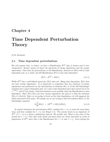
Chapter 4Time Dependent PerturbationTheoryc B. Zwiebach4.1Time dependent perturbationsWe will assume that, as before, we have a Hamiltonian H (0) that is known and is timeindependent. Known means we know the spectrum of energy eigenstates and the energyeigenvalues. This time the perturbation to the Hamiltonian, denoted as δH(t) will be timedependent and, as a result, the full Hamiltonian H(t) is also time dependentH(t) H (0) δH(t) .(4.1.1)While H (0) has a well-defined spectrum, H(t) does not. Being time dependent, H(t) doesnot have energy eigenstates. It is important to remember that the existence of energyeigenstates was predicated on the factorization of solutions Ψ(x, t) of the full Schrödingerequation into a space-dependent part ψ(x) and a time dependent part that turned out to bee iEt/ , with E the energy. Such factorization is not possible when the Hamiltonian is timedependent. Since H(t) does not have energy eigenstates the goal is to find the solutions Ψ(x, t)i directly. Since we are going to focus on the time dependence, we will suppress thelabels associated with space. We simply say we are trying to find the solution Ψ(t)i to theSchrödinger equation i Ψ(t)i H (0) δH(t) Ψ(t)i .(4.1.2) tIn typical situations the perturbation δH(t) vanishes for t t0 , it exists for some finitetime, and then vanishes for t tf (see Figure 4.1). The system starts in an eigenstate ofH (0) at t t0 or a linear combination thereof. We usually ask: What is the state of thesystem for t tf ? Note that both initial and final states are nicely described in terms ofeigenstates of H (0) since this is the Hamiltonian for t t0 and t tf . Even during the73
74CHAPTER 4. TIME DEPENDENT PERTURBATION THEORYFigure 4.1: Time dependent perturbations typically exist for some time interval, here from t0 to tf .time when the perturbation is on we can use the eigenstates of H (0) to describe the system,since these eigenstates form a complete basis, but the time dependence is very nontrivial.Many physical questions can be couched in this language. For example, assume we havea hydrogen atom in its ground state. We turn on EM fields for some time interval. We canthen ask: What are the probabilities to find the atom in each of the various excited statesafter the perturbation turned off?4.1.1The interaction pictureIn order to solve efficiently for the state Ψ(t)i we will introduce the Interaction Picture ofQuantum Mechanics. This picture uses some elements of the Heisenberg picture and someelements of the Schrödinger picture. We will use the known Hamiltonian H (0) to definesome Heisenberg operators and the perturbation δH will be used to write a Schrödingerequation.We begin by recalling some facts from the Heisenberg picture. For any Hamiltonian,time dependent or not, one can determine the unitary operator U(t) that generates timeevolution: Ψ(t)i U(t) Ψ(0)i .(4.1.3)The Heisenberg operator ÂH associated with a Schrödinger operator Âs is obtained byconsidering a rewriting of expectation values:hΨ(t) Âs Ψ(t)i hΨ(0) U † (t)Âs U(t) Ψ(0)i hΨ(0) ÂH Ψ(0)i ,(4.1.4)AH U † (t)Âs U(t) .(4.1.5)whereThis definition applies even for time dependent Schrödinger operators. Note that the operator U † brings states to rest:U † (t) Ψ(t)i U † (t)U(t) Ψ(0)i Ψ(0)i .(4.1.6)In our problem the known Hamiltonian H (0) is time independent and the associated unitarytime evolution operator U0 (t) takes the simple form iH (0) t U0 (t) exp . (4.1.7)
4.1. TIME DEPENDENT PERTURBATIONS75The state Ψ(t)i in our problem evolves through the effects of H (0) plus δH. Motivatedeby (4.1.6) we define the auxiliary ket Ψ(t)as the ket Ψ(t)i partially brought to rest(0)through H : iH (0) t eΨ(t) expΨ(t) .(4.1.8) eExpect that Schrödinger equation for Ψ(t)will be simpler, as the above must have takenecare of the time dependence generated by H (0) . Of cours, if we can determine Ψ(t)wecan easily get back the desired state Ψ(t) inverting the above relation to find iH (0) t eΨ(t).Ψ(t) exp (4.1.9)eOur objective now is to find the Schrödinger equation for Ψ(t). Taking the timederivative of (4.1.8) and using (4.1.2)i iH (0) t d eeΨ(t) H (0) Ψ(t)(H (0) δH(t)) Ψ(t) expdt "# iH (0) t iH (0) t (0)(0)e H exp(H δH(t)) exp Ψ(t) iH (0) t iH (0) t e expδH(t) exp Ψ(t),(4.1.10) where the dependence on H (0) cancelled out. We have thus found the Schrödinger equationi d efeΨ(t).Ψ(t) δH(t)dt(4.1.11)fwhere the operator δH(t)is defined as iH (0) t iH (0) t fδH(t) expδH(t) exp . (4.1.12)feNote that as expected the time evolution left in Ψ(t)is generated by δH(t)via a Schrödingerfequation. The operator δH(t)is nothing else but the Heisenberg version of δH generated(0)using H ! This is an interaction picture, a mixture of Heisenberg’s and Schrödinger picture. While we have some Heisenberg(0) operators there is still a time dependent stateeΨ(t)and a Schrödinger equation for it.
76CHAPTER 4. TIME DEPENDENT PERTURBATION THEORYHow does it all look in an orthonormal basis? Let ni be the complete orthonormal basisof states for H (0) :H (0) ni En ni .(4.1.13)This time there is no need for a (0) superscript, since neither the states nor their energieswill be corrected (there are no energy eigenstates in the time-dependent theory). We thenwrite an ansatz for our unknown ket:XeΨ(t) cn (t) ni .(4.1.14)nHere the functions cn (t) are unknown. This expansion is justified since the states ni forma basis, and thus at all times they can be used to describe the state of the system. Theoriginal wavefunction is then: iH (0) t XiEn te ni .(4.1.15)Ψ(t) exp Ψ(t) cn (t) exp nNote that the time dependence due to H (0) is present here. If we had δH 0 the stateeΨ(t)would be a constant, as demanded by the Schrödinger equation (4.1.11) and thecn (t) would be constants. The solution above would give the expected time evolution of thestates under H (0) .To see what the Schrödinger equation tells us about the functions cn (t) we plug theansatz (4.1.14) into (4.1.11):i Xd Xfcm (t) mi δH(t)cn (t) nidt mn(4.1.16)Using dots for time derivatives and introducing a resolution of the identity on the right-handside we findXXXfi ċm (t) mi mihm δH(t)cn (t) nimm Xn mim XXfhm δH(t) nicn (t)nf mn (t)cn (t) mi .δH(4.1.17)m,nHere we have used the familiar matrix element notationf mn (t) hm δH(t) nifδH.Equating the coefficients of the basis kets mi in (4.1.17) we get the equationsXf mn (t) cn (t) .i ċm (t) δHn(4.1.18)(4.1.19)
4.1. TIME DEPENDENT PERTURBATIONS77The Schrödinger equation has become an infinite set of coupled first-order differential equations. The matrix elements in the equation can be simplified a bit by passing to un-tildevariables: (0) (0) f mn (t) m exp iH t δH(t) exp iH t nδH i exp (Em En )t hm δH(t) ni . If we defineωmn Em En, (4.1.20)(4.1.21)we then havef mn (t) eiωmn t δHmn (t) .δH(4.1.22)The coupled equations (4.1.19) for the functions cn (t) then becomei ċm (t) Xeiωmn t δHmn (t)cn (t) .(4.1.23)n4.1.2Example (based on Griffiths Problem 9.3)Consider a two-state system with basis states ai and bi, eigenstates of H (0) with energiesEa and Eb , respectively. Callωab (Ea Eb )/ .(4.1.24)Now take the perturbation to be a matrix times a delta function at time equal zero. Thusthe perturbation only exists for time equal zero: 0 αδ(t) U δ(t) ,(4.1.25)δH(t) α 0where α is a complex number. With the basis vectors ordered as 1i ai and 2i bi wehave Uaa Uab U , with Uaa Ubb 0 and Uab Uba α.(4.1.26)Uba UbbThere is a sudden violent perturbation at t 0 with off-diagonal elements that shouldproduce transition. Take the system to be in ai for t , what is the probability thatit is in bi for t ?Solution: First note that if the system is in ai at t it will remain in state ai untilt 0 , that is, just before the perturbation turns on. This is because ai is an energyeigenstate of H (0) . In fact we have, up to a constant phase, Ψ(t)i e iEa t/ ai ,for t 0 .(4.1.27)
78CHAPTER 4. TIME DEPENDENT PERTURBATION THEORYWe are asked what will be the probability to find the state in bi at t , but in fact, theanswer is the same as the probability to find the state in bi at t 0 . This is because theperturbation does not exist anymore and if the state at t 0 is Ψ(0 )i γa ai γb bi ,(4.1.28)with γ1 and γ2 constants, then the state for any time t 0 will be Ψ(t)i γa aie iEa t/ γb bie iEb t/ .(4.1.29)The probability pb (t) to find the state bi at time t will bepb (t) hb Ψ(t)i 2 γb e iEb t/ γb 2 ,(4.1.30)and, as expected, this is time independent. It follows that to solve this problem we mustjust find the state at t 0 and determine the constants γ1 and γ2 .Since we have two basis states the unknown tilde state iseΨ(t) ca (t) ai cb (t) bi ,(4.1.31)and the initial conditions are stating that the system begins in the state ai areca (0 ) 1 ,cb (0 ) 0 .(4.1.32)The differential equations (4.1.23) take the formi ċa (t) eiωab t δHab (t)cb (t) ,i ċb (t) eiωba t δHba (t)ca (t) .(4.1.33)The couplings are off-diagonal because δHaa δHbb 0. Using the form of the δH matrixelements,i ċa (t) eiωab t α δ(t) cb (t) ,i ċb (t) e iωab t α δ(t) ca (t) .(4.1.34)We know that for functions f continuous at t 0 we have f (t)δ(t) f (0)δ(t). We nowask if we are allowed to use such identity for the right-hand side of the above equations. Infact we can use the identity for e iωab t but not for the functions ca (t) and cb (t) that, areexpected to be discontinuous at t 0. They must be so, because they can only change att 0, when the delta function exists. Evaluating the exponentials at t 0 we then get thesimpler equationsi ċa (t) α δ(t) cb (t) ,i ċb (t) α δ(t) ca (t) .(4.1.35)
4.1. TIME DEPENDENT PERTURBATIONS79With such singular right-hand sides, the solution of these equations needs regulation. Wewill regulate the delta function and solve the problem. A consistency check is that thesolution has a well-defined limit as the regulator is removed. We will replace the δ(t) bythe function t0 (t), with t0 0, defined as follows:(1/t0 , for t [0, t0 ] ,(4.1.36)δ(t) t0 (t) 0,otherwise .RNote that as appropriate, dt t0 (t) 1, and that t0 (t) in the limit as t0 0 approachesa delta function. If we replace the delta functions in (4.1.37) by the regulator we find, fort [0, t0 ]αFor t [0, t0 ] :i ċa (t) cb (t) ,t0(4.1.37)α i ċb (t) ca (t) .t0For any other times the right-hand side vanishes. By taking a time derivative of the firstequation and using the second one we find that α 21 α 1 α ca (t) ca (t) .(4.1.38)c̈a (t) i t0 i t0 t0This is a simple second order differential equation and its general solution is α t α t β1 sin.ca (t) β0 cos t0 t0(4.1.39)This is accompanied with cb (t) which is readily obtained from the first line in (4.1.37): α t α t i t0i α cb (t) ċa (t) β0 sin β1 cos.(4.1.40)αα t0 t0The initial conditions (4.1.32) tell us that in this regulated problem ca (0) 1 and cb (0) 0.Given the solutions above, the first condition fixes β0 1 and the second fixes β1 0. Thus,our solutions are: α tFor t [0, t0 ] :ca (t) cos,(4.1.41) t0 α α tcb (t) isin.(4.1.42)α t0When the (regulated) perturbation is turned off (t t0 ), ca and cb stop varying and theconstant value they take is their values at t t0 . Hence α ca (t t0 ) ca (t0 ) cos,(4.1.43) α α cb (t t0 ) cb (t0 ) isin.(4.1.44)α
80CHAPTER 4. TIME DEPENDENT PERTURBATION THEORYNote that these values are t0 independent. Being regulator independent, we can safely takethe limit t0 0 to get α ca (t 0) cos,(4.1.45) α α .(4.1.46)sincb (t 0) iα Our calculation above shows that at t 0 the state will be α α α e Ψ(0 )i Ψ(0 )i cosa isinb . α With only free evolution ensuing for t 0 we have (as anticipated in (4.1.29)) α α α iEa t/ a e ib e iEb t/ . Ψ(t)i cossin α (4.1.47)(4.1.48)The probabilities to be found in ai or in bi are time-independent, we are in a superpositionof energy eigenstates! We can now easily calculate the probability pb (t) to find the systemin bi for t 0 as well as the probability pa (t) to find the system in ai for t 0: α pb (t) hb Ψ(t)i 2 sin2, (4.1.49) 22 α pa (t) ha Ψ(t)i cos. Note that pa (t) pb (t) 1, as required. The above is the exact solution of this system. If wehad worked in perturbation theory, we would be taking the strength α of the interactionto be small. The answers we would obtain would form the power series expansion of theabove formulas in the limit as α / is small.4.2Perturbative solutionIn order to set up the perturbative expansion properly we include a unit-free small parameterλ multiplying the perturbation δH in the time-dependent Hamiltonian (4.1.1):H(t) H (0) λδH(t) .(4.2.1)eWith such a replacement the interaction picture Schrödinger equation for Ψ(t)iin (4.1.11)now becomesd efei Ψ(t) λδH(t)Ψ(t).(4.2.2)dteAs we did in time-independent perturbation theory we start by expanding Ψ(t)in powersof the parameter λ: ee (0) (t) λ Ψe (1) (t) λ2 Ψe (2) (t) O λ3 .Ψ(t) Ψ(4.2.3)
4.2. PERTURBATIVE SOLUTION81We now insert this into both sides of the Schrödinger equation (4.2.2), and using t for timederivatives, we find e (0) (t) λ i t Ψe (1) (t) λ2 i t Ψe (2) (t) λ3 i t Ψe (2) (t) O λ4i t Ψ f Ψf Ψf Ψe (2) (t) O λ4 .e (1) (t) λ3 δHe (0) (t) λ2 δH λ δH(4.2.4)The coefficient of each power of λ must vanish, giving use (0) (t)i t Ψ 0,e (1) (t)i t Ψf Ψe (0) (t) , δHe (2) (t)i t Ψf Ψe (1) (t) , δH.e (n 1) (t)i t Ψ(4.2.5). f Ψe (n) (t) . δHThe origin of the pattern is clear. Since the Schrödinger equation has an explicit λ multifplying the right-hand side, the time derivative of the n-th component is coupled to the δHperturbation acting on the (n 1)-th component.Let us consider the initial condition in detail. We will assume that the perturbationturns on at t 0, so that the initial condition is given in terms of Ψ(0)i. Since oureSchrödinger equation is in terms of Ψ(t)iwe use the relation ((4.1.8)) between them toconclude that both tilde and un-tilde wavefunctions are equal at t 0:e Ψ(0)i Ψ(0)i .(4.2.6)Given this, the expansion (4.2.3) evaluated at t 0 implies that:eΨ(0)e (0) (0) Ψ(0)i Ψe (1) (0) λ Ψe (2) (0) λ2 Ψ O λ3 .(4.2.7)This must be viewed, again, as an equation that holds for all values of λ. As a result, thecoefficient of each power of λ must vanish and we havee (0) (0)Ψ Ψ(0) ,e (n) (0)Ψ 0,(4.2.8)n 1, 2, 3 . . . .These are the relevant initial conditions.e (0) (t) is time independent.Consider now the first equation in (4.2.5). It states that ΨThis is reasonable: if the perturbation vanishes, this is the only equation we get and weee (0) (t) and the initialshould expect Ψ(t)constant. Using the time-independence of Ψcondition we havee (0) (t) Ψe (0) (0) Ψ(0) ,Ψ(4.2.9)
82CHAPTER 4. TIME DEPENDENT PERTURBATION THEORYand we have solved the first equation completely:e (0) Ψ(0) .Ψ(4.2.10)Using this result, the O(λ) equation reads:f Ψfe (1) (t) δHe (0) (t) δH(t)i t ΨΨ(0) .(4.2.11)The solution can be written as an integral:tZe (1) (t) Ψ0f 0)δH(tΨ(0) dt0 .i (4.2.12)Note that by setting the lower limit of integration at t 0 we have implemented correctlye (1) (0)i 0. The next equation, of order λ2 reads:the initial condition Ψf Ψe (2) (t) δHe (1) (t) ,i t Ψ(4.2.13)and its solution ise (2) (t) ΨZ0tf 0)δH(te (1) (t0 ) dt0 ,Ψi (4.2.14)e (1) (t0 ) we nowconsistent with the initial condition. Using our previous result to write Ψhave an iterated integral expression:e (2) (t) ΨZ0tf 00 )f 0 ) Z t0 δH(tδH(tdt0Ψ(0) dt00 .i i 0(4.2.15)It should be clear from this discussion how to write the iterated integral expression fore (k) (t) , with k 2. The solution, setting λ 1 and summarizing is thenΨ! iH (0) t e (1) (t)i Ψe (2) (t)i · · · Ψ(0)i Ψ(4.2.16)Ψ(t) exp Let us use our perturbation theory to calculate the probability Pm n (t) to transitionfrom ni at t 0 to mi, with m 6 n, at time t, under the effect of the perturbation. Bydefinition2Pm n (t) hm Ψ(t)i .(4.2.17)Using the tilde wavefunction, for which we know how to write the perturbation, we havePm n (t) hm e iH(0) t/ eΨ(t)22e hm Ψ(t)i,(4.2.18)
4.2. PERTURBATIVE SOLUTION83since the phase that arises from the action on the bra vanishes upon the calculation of theenorm squared. Now using the perturbation expression for Ψ(t)i(setting λ 1) we havePm n (t) hm e (1) (t) Ψe (2) (t) . . .Ψ(0) Ψ 2.(4.2.19)Since we are told that Ψ(0)i ni and ni is orthogonal to mi we finde (1) (t) hm Ψe (2) (t) . . .Pm n (t) hm Ψ2.(4.2.20)To first order in perturbation theory we only keep the first term in the sum and using oure (1) (t)i we findresult for Ψ(1)Pm n(t)Z hm 0tf 0)δH(t ni dt0i 2Z 0tf 0 ) nihm δH(tdt0i 2.(4.2.21)f and those of δH we finally haveRecalling the relation between the matrix elements of δHour result for the transition probability to first order in perturbation theory:(1)Pm n(t)tZ0eiωmn t 0δH mn (t0 ) 0dti 2.(4.2.22)This is a key result and will be very useful in the applications we will consider.Exercise: Prove the remarkable equality of transition probabilities(1)(1)Pm n(t) Pn m(t) ,(4.2.23)valid to first order in perturbation theory.It will also be useful to have our results in terms of the time-dependent coefficients cn (t)introduced earlier through the expansionXeΨ(t) cn (t) ni .(4.2.24)neSince Ψ(0) Ψ(0)the initial condition readsΨ(0) Xe (0) (0) ,cn (0) ni Ψ(4.2.25)nwhere we also used (4.2.9). In this notation, the cn (t) functions also have a λ expansion,because we writeXe (k) (t) Ψc(k)k 0, 1, 2, . . .(4.2.26)n (t) ni ,n
84CHAPTER 4. TIME DEPENDENT PERTURBATION THEORYand therefore the earlier relationeΨ(t)e (0) (t) Ψe (1) (t) λ Ψe (2) (t) λ2 Ψ O λ3 .(4.2.27)now gives(1)2 (2)cn (t) c(0)n (t) λcn (t) λ cn (t) . . .(4.2.28)e (0) (t)i is in fact constant we haveSince Ψ(0)c(0)n (t) cn (0) cn (0) ,(4.2.29)where we used (4.2.25). The other initial conditions given earlier in (4.2.8) imply thatc(k)n (0) 0 ,k 1, 2, 3 . . . .(4.2.30)e (1) (t) we haveTherefore, using our result (4.2.12) for Ψe (1) (t) ΨXc(1)n (t) ni tZ0nXf 0)δH(tdt0cn (0) ni ,i n(4.2.31)f 0 ) nihm δH(tcn (0) dt0 .i (4.2.32)and as a result,c(1)m (t)e (1) (t) hm ΨXZn0tWe therefore havec(1)m (t) XZ0nt0dt0 eiωmn tδHmn (t0 )cn (0) .i (4.2.33)The probability Pm (t) to be found in the state mi at time t isePm (t) hm Ψ(t)i 2 hm Ψ(t)i2 cm (t) 2 .(4.2.34)To first order in perturbation theory the answer would be (with λ 1)(1)Pm(t) cm (0) c(1)m (t)22(1) 2 cm (0) cm (0) c(1)m (t) cm (t) cm (0) O(δH ) .(1)(4.2.35)Note that the cm (t) 2 term cannot be kept to this order of approximation, since it is of(2)the same order as contributions that would arise from cm (t).
4.2. PERTURBATIVE SOLUTION4.2.185Example NMRThe Hamiltonian for a particle with a magnetic moment inside a magnetic field can bewritten in the formH ω · S,(4.2.36)where S is the spin operator and ω is precession angular velocity vector, itself a functionof the magnetic field. Note that the Hamiltonian has properly units of energy (ω ). Let ustake the unperturbed Hamiltonian to beH (0) ω0 Sz 2ω0 σz .(4.2.37)For NMR applications one has ω0 500 Hz and this represents the physics of a magneticfield along the z axis. Let us now consider some possible perturbations.Case 1: Time independent perturbation Let us consider adding at t 0 a constantperturbation associated with an additional small uniform magnetic field along the x axis:H H (0) δH , with δH ΩSx ,(4.2.38)For this to be a small perturbation we will takeΩ ω0 .(4.2.39)Hence, for the full Hamiltonian H we have ω (Ω, 0, ω0 )H (Ω, 0, ω0 ) ·(Sx , Sy , Sz ) {z }(4.2.40)ωThe problem is simple enough that an exact solution is possible. The perturbed HamiltonianωH has energy eigenstates n; i, spin states that point with n ω with energies 2 ω .These eigenstates could be recovered using time-independent non-degenerate perturbationtheory using Ω/ω0 as a small parameter and starting with the eigenstates i of H (0) .In time-dependent perturbation theory we obtain the time-dependent evolution of initialstates as they are affected by the perturbation. Recalling (4.2.12) we haveZ t f 0δH(t )e (1) (t) Ψ(0) dt0(4.2.41)Ψi 0
86CHAPTER 4. TIME DEPENDENT PERTURBATION THEORYf requires a bit of computation. One quickly finds thatThe calculation of δHh h σz iσz ifΩŜx exp iω0 t Ω Ŝx cos ω0 t Ŝy sin ω0 t .δH(t) exp iω0 t22(4.2.42)As a result we set:Z t e (1) (t) ΩΨŜx cos ω0 t0 Ŝy sin ω0 t0 Ψ(0) dt0i 0 i1 Ω h Ŝx sin ω0 t cos(ω0 t0 ) 1 Ŝy Ψ(0) .i ω0(4.2.43)As expected, the result is first order in the small parameter Ω/ω0 . Following (4.2.16) thetime-dependent state is, to first approximation!hi σz i1 Ω hΨ(t) exp iω0 t1 Ŝx sin ω0 t cos(ω0 t0 ) 1 Ŝy Ψ(0)i2i ω0(4.2.44) O((Ω/ω0 )2 ) .Physically the solution is clear. The original spin state Ψ(0) precesses about the directionof ω with angular velocity ω.Case 2: Time dependent perturbation. Suppose that to the original Hamiltonian weadd the effect of a rotating magnetic field, rotating with the same angular velocity ω0 thatcorresponds to the Larmor frequency of the original Hamiltonian: δH(t) Ω Ŝx cos ω0 t Ŝy sin ω0 t .(4.2.45)f we can use (4.2.42) with t replaced by t so that theTo compute the perturbation δHright-hand side of this equation is proportional to δH:hh σz iσz iexp iω0 tΩŜx exp iω0 t Ω Ŝx cos ω0 t Ŝy sin ω0 t .(4.2.46)22Moving the exponentials on the left-hand side to the right-hand side we findh hσz i σz iΩŜx exp iω0 tΩ Ŝx cos ω0 t Ŝy sin ω0 t exp iω0 t.22(4.2.47)f Thus we have shown thatThe right-hand side is, by definition, δH.fδH(t) ΩŜx ,(4.2.48)is in fact a time-independent Hamiltonian. This means that the Schrödinger equation fore is immediately solvedΨeΨ(t) f δHt e exp iΨ(0) ΩŜx t exp iΨ(0) . (4.2.49)
4.3. FERMI’S GOLDEN RULE87The complete and exact answer is thereforeh iH (0) t ihhσz iσx ieΨ(t) exp exp iΩtΨ(0) .Ψ(t) exp iω0 t 22(4.2.50)This is a much more non trivial motion! A spin originally aligned along ẑ will spiral intothe x, y plane with angular velocity Ω.4.3Fermi’s Golden RuleLet us now consider transitions where the initial state is part of a discrete spectrum but thefinal state is part of a continuum. The ionization of an atom is perhaps the most familiarexample: the initial state may be one of the discrete bound states of the atom while thefinal state includes a free electron a momentum eigenstate that is part of a continuum ofnon-normalizable states.As we will see, while the probability of transition between discrete states exhibits periodic dependence in time, if the final state is part of a continuum an integral over finalstates is needed and the result is a transition probability linear in time. To such probabilityfunction we will be able to associate a transition rate. The final answer for the transitionrate is given by Fermi’s Golden Rule.We will consider two different cases in full detail:1. Constant perturbations. In this case the perturbation, called V turns on at t 0 butit is otherwise time independent:H (H (0) ,H (0) Vfor t 0 ,(4.3.1)for t 0 .This situation is relevant for the phenomenon of auto-ionization, where an internaltransition in the atom is accompanied by the ejection of an electron.
88CHAPTER 4. TIME DEPENDENT PERTURBATION THEORY2. Harmonic perturbations. In this case the time dependence of the perturbation δH isperiodic, namely,H(t) H (0) δH(t) ,(4.3.2)with(δH(t) for t 0 ,0,2H 0 cos ωt ,(4.3.3)for t 0 .Note the factor of two entering the definition of δH in terms of the time independentH 0 . This situation is relevant to the interaction of electromagnetic fields with atoms.Before starting with the analysis of these two cases let us consider the way to dealwith continuum states, as the final states in the transition will belong to a continuum.The fact is that we need to be able to count the states in the continuuum, so we willreplace infinite space by a very large cubic box of side length L and we will impose periodicboundary conditions on the wavefunctions. The result will be a discrete spectrum wherethe separation between the states can be made arbitrarily small, thus simulating accuratelya continuum in the limit L . If the states are energetic enough and the potential isshort range, momentum eigenstates are a good representation of the continuum.To count states use a large box, which can be taken to be a cube of side L:We call L a regulator as it allows us to deal with infinite quantities (like the volume ofspace or the number of continuum states). At the end of our calculations the value of Lmust drop out. This is a consistency check. The momentum eigenstates ψ(x take the form1ψ(x) eikx x eiky y eikz z ,L3with constant k (kx , ky , kz ). It is clear that the states are normalized correctlyZZ12 3 ψ(x) d x 3 d3 x 1 .Lbox(4.3.4)(4.3.5)The k 0 s are quantized by the periodicity condition on the wavefunction:ψ(x L, y, z) ψ(x, y L, z) ψ(x, y, z L) ψ(x, y, z) .(4.3.6)The quantization giveskx L 2πnx Ldkx 2πdnx ,ky L 2πny Ldky 2πdny ,kz L 2πnz Ldkz 2πdnz .(4.3.7)
4.3. FERMI’S GOLDEN RULE89Define N as the total number of states within the little cubic volume element d3 k. Itfollows from (4.3.7) that we have 3L N dnx dny dnz d3 k .(4.3.8)2πNote that N only depends on d3 k and not on k itself: the density of states is constant inmomentum space.Now let d3 k be a volume element determined in spherical coordinates k, θ, φ and byranges dk, dθ, dφ. Therefored3 k k 2 dk sin θdθ dφ k 2 dk dΩ(4.3.9)We now want to express the density of states as a function of energy. For this we takedifferentials of the relation between the wavenumber k and the energy E:E Back in (4.3.9) we have 2 k 22m kdk mdE . 2mdE dΩ , 2 3Lm N k 2 dΩ dE .2π d3 k khence(4.3.10)(4.3.11)(4.3.12)We now equate N ρ(E)dE ,(4.3.13)where ρ(E) is a density of states, more precisely, it is the number of states per unit energyat around energy E and with momentum pointing within the solid angle dΩ. The last twoequations determine for us this density:ρ(E) L3 mk dΩ .8π 3 2(4.3.14)With a very large box, a sum over states can be replaced by an integral as followsZX··· · · · ρ(E)dE(4.3.15)stateswhere the dots denote an arbitrary function of the momenta k of the states.
90CHAPTER 4. TIME DEPENDENT PERTURBATION THEORY4.3.1Constant transitions.The Hamiltonian, as given in (4.3.1) takes the form( (0)Hfor t 0H H (0) V for t 0 .(4.3.16)We thus identify δH(t) V for t 0. Recalling the formula (4.2.33) for transition amplitudes to first order in perturbation theory we haveXZ t0 Vmndt0 eiωmn tc(1)(t) cn (0) .(4.3.17)mi 0nTo represent an initial state i at 0 we take cn (0) δn,i . For a transition to a final statef at time t0 we set m f and we have an integral that is easily performed:(1)cf (t0 )1 i Zt00iωf i t0Vf i e0Vf i eiωf i tdt i iωf it00(4.3.18)0Evaluating the limits and simplifying(1)cf (t0 ) V eiωf i t0 /2Vf i ωf i t0fiiωf i t0 1 e ( 2i) sin.Ef EiEf Ei2(4.3.19)(1)The transition probability to go from i at t 0 to f at t t0 is then cf (t0 ) 2 and istherefore ω t4 sin2 f2i 0Pf i (t0 ) Vf i 2.(4.3.20)(Ef Ei )2This first order result in perturbation theory is expected to be accurate at time t0 ifPf i (t0 ) 1. Certainly a large transition probability at first order could not be trustedand would require examination of higher orders.To understand the main features of the result for the transition probability we examinehow it behaves for different values of the final energy Ef . If Ef 6 Ei the transition is saidto be energy non-conserving. Of course, energy is conserved overall, as it would be suppliedby the perturbation. If Ef Ei we have an energy conserving transition. Both are possibleand let us consider them in turn.1. Ef 6 Ei . In this case the transition probability Pf i (t0 ) as a function of t0 is shownin Figure 4.2. The behavior is oscillatory with frequency ωf i . If the amplitude of theoscillation is much less than one4 Vf i 21(Ef Ei )2(4.3.21)
4.3. FERMI’S GOLDEN RULE91Figure 4.2: The transition probability as a function of time for constant perturbations.then this first order transition probability Pf i (t0 ) is accurate for all times t0 as it isalways small. The amplitude is suppressed as Ef Ei grows, due to the factor inthe denominator. This indicates that the larger the energy ‘violation’ the smaller theprobability of transition. This is happening because a perturbation that turns on andthen remains constant is not an efficient supply of energy.2. Ef Ei . In this limit ωf i approaches zero and therefore (Ef Ei )2 22 ωf i t0sin't0 .24 2(4.3.22)It follows from (4.3.20) thatlim Pf i (t0 ) Ef Ei Vf i 2 2t . 2 0(4.3.23)The probability for an energy-conserving transition grows quadratically in time, anddoes so without bound! This result, however, can only be trusted for small enough t0such that Pf i (t0 ) 1.Note that a quadratic growth of Pf i is also visible in the energy non-conserving Ef 6 Ei case for very small times t0 . Indeed, (4.3.20) leads again to limt0 0 Pf i (t0 ) Vf i 2 t20 / 2 , while Ef 6 Ei . This behavior can be noted near the origin in Figure 4.2.Our next step is to integrate the transition probability over the now discretized continuum of final states. Remarkably, upon integration the oscillatory and quadratic behaviorsof the transition probability as a function of time will conspire to create a linear behavior!The sum of tran
74 CHAPTER 4. TIME DEPENDENT PERTURBATION THEORY Figure 4.1: Time dependent perturbations typically exist for some time interval, here from t 0 to f. time when the perturbation is on we can use the eigenstates of H(0) to describe the system, since these eigenstates form a complete basis, but the time dependence is very nontrivial.