Transcription
Chapter 1Knowledge Discovery and DataMining: Concepts and FundamentalAspects1.1OverviewThe goal of this chapter is t o summarize the preliminary backgroundrequired for this book. The chapter provides an overview of concepts fromvarious interrelated fields used in the subsequent chapters. It starts bydefining basic arguments from data mining and supervised machine learning. Next, there is a review on some common induction algorithms anda discussion on their advantages and drawbacks. Performance evaluationtechniques are then presented and finally, open challenges in the field arediscussed.1.2Data Mining and Knowledge DiscoveryData mining is the science and technology of exploring data in order t odiscover previously unknown patterns. Data Mining is a part of the overallprocess of Knowledge Discovery in databases (KDD). The accessibility andabundance of information today makes data mining a matter of considerableimportance and necessity.Most data mining techniques are based on inductive learning (see[Mitchell (1997)]), where a model is constructed explicitly or implicitly by generalizing from a sufficient number of training examples. Theunderlying assumption of the inductive approach is that the trained modelis applicable t o future, unseen examples. Strictly speaking, any form ofinference in which the conclusions are not deductively implied by thepremises can be thought of as induction.Traditionally data collection is considered to be one of the mostimportant stages in data analysis. An analyst (e.g., a statistician) used
2Decomposition Methodology for Knowledge Discovery and Data Miningthe available domain knowledge to select the variables to be collected. Thenumber of variables selected was usually small and the collection of theirvalues could be done manually (e.g., utilizing hand-written records or oralinterviews). In the case of computer-aided analysis, the analyst had t o enter the colIected data into a statistical computer ackageor an electronicspreadsheet. Due to the high cost of data collection, people learned to makedecisions based on limited information.However, since the information-age, the accumulation of data becomeeasier and storing it inexpensive. It has been estimated that the amountof stored information doubles every twenty months [Frawley et al. (1991)).Unfortunately, as the amount of machine readable information increases,the ability to understand and make use of it does not keep pace with itsgrowth. Data mining is a term coined to describe the process of siftingthrough large databases in search of interesting patterns and relationships.Practically, Data Mining provides tools by which large quantities of datacan be automatically analyzed. Some of the researchers consider the term"Data Mining" as misleading and prefer the term "Knowledge Mining" asit provides a better analogy to gold mining [Klosgen and Zytkow (2002)l.The Knowledge Discovery in Databases (KDD) process was defined mymany, for instance [Fayyad et al. (1996)l define it as "the nontrivial processof identifying valid, novel, potentially useful, and ultimately understandablepatterns in data". [Friedman (1997a)l considers the KDD process as anautomatic exploratory data analysis of large databases. [Hand (1998)] viewsit as a secondary data analysis of large databases. The term "Secondary"emphasizes the fact that the primary purpose of the database was not dataanalysis. Data Mining can be considered as a central step of the overallprocess of the Knowledge Discovery in Databases (KDD) process. Due tothe centrality of data mining in the KDD process, there are some researchersand practitioners that use the term "data mining" as synonymous to thecomplete KDD process.Several researchers, such as [ r a c h m a nand Anand (1994)], [ a a det al. (1996)], a aim on and Last (2000)] and [Reinartz (2002)l have proposed different ways to divide the KDD process into phases. This bookadopts a hybridization of these proposals and suggests breaking the KDDprocess into the following eight phases. Note that the process is iterativeand moving back to previous phases may be required.(1) Developing an understanding of the application domain, the relevantprior knowledge and the goals of the end-user.
Concepts and Fundamental Aspects3(2) Selecting a data set on which discovery is to be performed.(3) Data Preprocessing: This stage includes operations for DimensionReduction (such as Feature Selection and Sampling), Data Cleansing(such as Handling Missing Values, Removal of Noise or Outliers), andData Transformation (such as Discretization of Numerical Attributesand Attribute Extraction)(4) Choosing the appropriate Data Mining task such as: classification,regression, clustering and summarization.(5) Choosing the Data Mining algorithm: This stage includes selecting thespecific method to be used for searching patterns.(6) Employing The Data mining Algorithm.(7) Evaluating and interpreting the mined patterns.(8) Deployment: Using the knowledge directly, incorporating the knowledge into another system for further action or simply documenting thediscovered knowledge.1.3Taxonomy of Data Mining MethodsIt is useful to distinguish between two main types of data mining: verification-oriented (the system verifies the user's hypothesis) anddiscovery-oriented (the system finds new rules and patterns autonomously)[Fayyad et al. (1996)l. Figure 1.1 illustrates this taxonomy.Discovery methods are methods that automatically identify patterns inthe data. The discovery method branch consists of prediction methodsversus description methods. Description-oriented Data Mining methodsfocus on (the part of) understanding the way the underlying data operates,where prediction-oriented methods aim to build a behavioral model thatcan get newly and unseen samples and is able to predict values of one ormore variables related to the sample.However, some prediction-oriented methods can also help provideunderstanding of the data.Most of the discovery-oriented techniques are based on inductive learning [Mitchell (1997)], where a model is constructed explicitly or implicitly by generalizing from a sufficient number of training examples . Theunderlying assumption of the inductive approach is that the trained modelis applicable to future unseen examples. Strictly speaking, any form of inference in which the conclusions are not deductively implied by the premisescan be thought of as induction.
4Decomposition Methodology for Knowledge Discovery and Data MiningGoodness of fitFig. 1.1 Taxonomy of Data Mining MethodsVerification methods, on the other hand, deal with evaluation of ahypothesis proposed by an external source (like an expert etc.). Thesemethods include the most common methods of traditional statistics, likegoodness-of-fit test, t-test of means, and analysis of variance. These methods are less associated with data mining than their discovery-orientedcounterparts because most data mining problems are concerned withselecting a hypothesis (out of a set of hypotheses) rather than testing aknown one. The focus of traditional statistical methods is usually on modelestimation as opposed to one of the main objectives of data mining: modelidentification [Elder and Pregibon (1996)l.1.41.4.1Supervised MethodsOverviewAnother common terminology used by the machine-learning communityrefers to the prediction methods as supervised learning as opposed to unsupervised learning. Unsupervised learning refers to modeling the distributionof instances in a typical, high-dimensional input space.
Concepts and Fundamental Aspects5According to [Kohavi and Provost (1998)] the term "Unsupervised learning" refers t o LLlearningtechniques that group instances without a prespecified dependent attribute". Thus the term unsurprised learning covers onlya portion of the description methods presented in Figure 1.1, for instance itdoes cover clustering methods but it does not cover visualization methods.Supervised methods are methods that attempt to discover the relationship between input attributes (sometimes called independent variables) anda target attribute (sometimes referred t o as a dependent variable). Therelationship discovered is represented in a structure referred to as a Model.Usually models describe and explain phenomena, which are hidden in thedataset and can be used for predicting the value of the target attributeknowing the values of the input attributes. The supervised methods canbe implemented on a variety of domains such as marketing, finance andmanufacturing.It is useful to distinguish between two main supervised models: Classification Models (Classifiers) and Regression Models. Regression modelsmap the input space into a real-valued domain. For instance, a regressor can predict the d e m q d for a certain product given it characteristics.On the other hand classifiers map the input space into predefined classes.For instance classifiers can be used t o classify mortgage consumers to good(fully payback the mortgage on time) and bad (delayed payback). Thereare many alternatives to represent classifiers, for example: Support VectorMachines, decision trees, probabilistic summaries, algebraic function, etc.This book deals mainly in classification problems. Along with regression and probability estimation, classification is one of the most studiedapproaches, possibly one with the greatest practical relevance. The potential benefits of progress in classification are immense since the techniquehas great impact on other areas, both within data mining and in its applications.1.4.2Training SetIn a typical supervised learning scenario, a training set is given and thegoal is to form a description that can be used to predict previously unseenexamples.The training set can be described in a variety of languages. Most frequently, it is described as a Bag Instance of a certain Bag Schema. ABag Instance is a collection of tuples (also known as records, rows or instances) that may contain duplicates. Each tuple is described by a vector of
6Decomposition Methodology for Knowledge Discovery and Data Miningattribute values. The bag schema provides the description of the attributesand their domains. For the purpose of this book, a bag schema is denotedas B(AU y) where A denotes the set of input attributes containing n attributes: A {al, . . . , a,, . . . , a,) and y represents the class variable or thetarget attribute.Attributes (sometimes called field, variable or feature) are typicallyone of two types: nominal (values are members of an unordered set), ornumeric (values are real numbers). When the attribute a, is nominal it , domain)l)valis useful to denote by dom(a,) {v,,l,v,,z,. . . , , , l d ( itsues, where (dom(a,)( stands for its finite cardinality. In a similar way, ( the) domain )of the target attribute.dom(y) {cl, . . . , c representsNumeric attributes have infinite cardinalities.The instance space (the set of all possible examples) is defined as aCartesian product of all the input attributes domains: X dom(al) xdom(az) x . . . x dom(a,). The Universal Instance Space (or the LabeledInstance Space) U is defined as a Cartesian product of all input attributedomains and the target attribute domain, i.e.: U X x dom(y).The training set is a Bag Instance consistin ofa set of m tuples. Formally the training set is denoted as S ( B ) ( ( x l , yl), . . . , (x,, y,)) wherex, E X and y, E dom(y).Usually, it is assumed that the training set tuples are generated randomly and independently according t o some fixed and unknown joint probability distribution D over U . Note that this is a generalization of the deterministic case when a supervisor classifies a tuple using a function y f (x).This book uses the common notation of bag algebra t o present projection (T) and selection ( a ) of tuples ([Grumbach and Milo (1996)].For example given the dataset S presented in Table 1.1, the expressionTa,,asUal nYesnANDa4 6Sresult with the dataset presented in Table 1.2.1.4.3Definition of the Classification ProblemThis section defines the classification problem. Originally the machinelearning community has introduced the problem of concept learning. Concepts are mental categories for objects, events, or ideas that have a common set of features. According t o [Mitchell (1997)l: "each concept canbe viewed as describing some subset of objects or events defined over alarger set" (e.g., the subset of a vehicle that constitues trucks). To learn aconcept is to infer its general definition from a set of examples. This definition may be either explicitly formulated or left implicit, but either way it
Concepts and Fundamental AspectsTable 1.1 Illustration of a Dataset Shaving five 116616414512356258679922221543Y010001100Table 1.2 The Result of the Expression a 2 , a 3 a l c c y e s ' Ls Based D 4 on, 6 theTable 1.1.assigns each possible example t o the concept or not. Thus, a concept can beregarded as a function from the Instance space t o the Boolean set, namely:c : X - {-1,l). Alternatively one can refer a concept c as a subset of X ,namely: {x E X : c ( x ) 1). A concept class C is a set of concepts.To learn a concept is t o infer its general definition from a set of examples.This definition may be either explicitly formulated or left implicit, buteither way it assigns each possible example to the concept or not. Thus, aconcept can be formally regarded as a function from the set of all possibleexamples to the Boolean set {True, False).Other communities, such as the KDD community prefer t o deal with astraightforward extension of Concept Learning, known as The ClasszjicationProblem. In this case we search for a function that maps the set of allpossible examples into a predefined set of class labels which are not limitedto the Boolean set. Most frequently the goal of the Classifiers Inducers isformally defined as:Given a training set S with input attributes set A {al, aa, . . . ,a,)and a nominal target attribute y from an unknown fixed distribution Dover the labeled instance space, the goal is to induce an optimal classifierwith minimum generalization error.
8Decomposition Methodology for Knowledge Discovery and Data MiningThe Generalization error is defined as the misclassification rate over thedistribution D. In case of the nominal attributes it can be expressed as:where L(y, I ( S ) ( x ) is the zero one loss function defined as:In case of numeric attributes the sum operator is replaced with theintegration operator.Consider the training set in Table 1.3 containing data concerning aboutten customers. Each customer is characterized by three attributes: Age,Gender and "Last Reaction" (an indication whether the customer has positively responded t o the last previous direct mailing campaign). The lastattribute ("Buy") describes whether that customer was willing to purchasea product in the current campaign. The goal is to induce a classifierthat most accurately classifies a potential customer t o LLBuyers"and "NonBuyers" in the current campaign, given the attributes: Age, Gender, LastReaction.Table 1.3 An Illustration of Direct Mailing Dataset.I Aae1.4.4I GenderI Last ReactionI BrivIInduction AlgorithmsAn Induction algorithm, or more concisely an Inducer (also known aslearner), is an entity that obtains a training set and forms a model that
Concepts and Fundamental Aspects9generalizes the relationship between the input attributes and the targetattribute. For example, an inducer may take as an input specific trainingtuples with the corresponding class label, and produce a classifier.The notation I represents an inducer and I ( S ) represents a model whichwas induced by performing I on a training set S . Using I(S) it is possibleto predict the target value of a tuple x,. This prediction is denoted asI(S)(xq).Given the long history and recent growth of the field, it is not surprising that several mature approaches to induction are now available t o thepractitioner.Classifiers may be represented differently from one inducer to another.For example, C4.5 [Quinlan (1993)] represents model as a decision treewhile Na'ive Bayes [ u d anda Hart (1973)] represents a model in the formof probabilistic summaries. Furthermore, inducers can be deterministic (asin the case of C4.5) or stochastic (as in the case of back propagation)The classifier generated by the inducer can be used t o classify an unseentuple either by explicitly assigning it t o a certain class (Crisp Classifier) orby providing a vector of probabilities representing the conditional probability of the given instance t o belong to each class (Probabilistic Classifier).Inducers that can construct Probabilistic Classifiers are known as Probabilistic Inducers. In this case it is possible to estimate the conditional probability PI(S)(y cj la, xq,i ; i 1 , . . . , n) of an observation x,. Note theaddition of the "hat" - - t o the conditional probability estimation isused for distinguishing it from the actual conditional probability.The following sections briefly review some of the major approachest o concept learning: Decision tree induction, Neural Networks, GeneticAlgorithms, instance- based learning, statistical methods, Bayesian methods and Support Vector Machines. This review focuses more on methodsthat have the greatest attention in this book.1.5Rule InductionRule induction algorithms generate a set of if-then rules that jointly represent the target function. The main advantage that rule induction offers isits high comprehensibility. Most of the Rule induction algorithms are basedon the separate and conquer paradigm [Michalski (1983)]. For that reasonthese algorithms are capable of finding simple axis parallel frontiers, arewell suited t o symbolic domains, and can often dispose easily of irrelevant
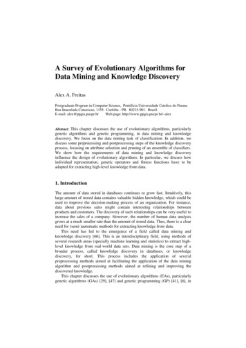
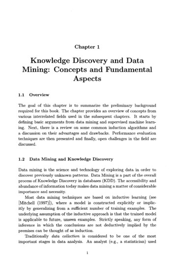
10Decomposition Methodology for Knowledge Discovery and Data Miningattributes; but they can have difficulty with nonaxisparallel frontiers, andsuffer from the fragmentation problem (i.e., the available data dwindles asinduction progresses [Pagallo and Huassler (1990)] and the small disjunctsproblem i.e., rules covering few training examples have a high error rate[Holte et al. (1989)l.1.6 Decision TreesA Decision tree is a classifier expressed as a recursive partition of theinstance space. A decision tree consists of nodes that form a Rooted Tree,meaning it is a Directed Tree with a node called root that has no incomingedges. All other nodes have exactly one incoming edge. A node with outgoing edges is called internal node or test nodes. All other nodes are calledleaves (also known as terminal nodes or decision nodes).In a decision tree, each internal node splits the instance space into twoor more subspaces according t o a certain discrete function of the inputattributes values. In the simplest and most frequent case each test considersa single attribute, such that the instance space is partitioned according tothe attribute's value. In the case of numeric attributes the condition refersto a range.Each leaf is assigned to one class representing the most appropriatetarget value. Usually the most appropriate target value is the class withthe greatest representation, because selecting this value minimizes the zeroone loss. However if a different loss function is used then a different classmay be selected in order t o minimize the loss function. Alternatively theleaf may hold a probability vector indicating the probability of the targetvalue having a certain value.Instances are classified by navigating them from the root of the treedown to a leaf, according to the outcome of the tests along the path.Figure 1.2 describes a decision tree t o the classification problem illustrated in Table 1.3 (whether or not a potential customer will respond toa direct mailing). Internal nodes are represented as circles whereas leavesare denoted as triangles. The node "Last R" stands for the attribute "LastReaction". Note that this decision tree incorporates both nominal andnumeric attributes. Given this classifier, the analyst can predict theresponse of a potential customer (by sorting it down the tree), and understand the behavioral characteristics of the potential customers regardingdirect mailing. Each node is labeled with the attribute it tests, and its
Concepts and Fundamental Aspects11branches are labeled with its corresponding values.In case of numeric attributes, decision trees can be geometrically interpreted as a collection of hyperplanes, each orthogonal t o one of the axes.Fig. 1.2 Decision Tree Presenting Response to Direct MailingNaturally, decision makers prefer a less complex decision tree, as itis considered more comprehensible. Furthermore, according to [Breimanet al. (1984)] the tree complexity has a crucial effect on its accuracy performance. Usually large trees are obtained by over fitting the data and henceexhibit poor generalization ability. Nevertheless a large decision tree canbe accurate if it was induced without over fitting the data. The tree complexity is explicitly controlled by the stopping criteria used and the pruningmethod employed. Usually the tree complexity is measured by one of thefollowing metrics: The total number of nodes, Total number of leaves, Tree
Decomposition Methodology for Knowledge Discovery and Data Mining12Depth and Number of attributes used.Decision tree induction is closely related to rule induction. Each pathfrom the root of a decision tree t o one of its leaves can be transformed intoa rule simply by conjoining the tests along the path to form the antecedentpart, and taking the leaf's class prediction as the class value. For example,one of the paths in Figure 1.2 can be transformed into the rule: "If customerage 5 30, and the gender of the customer is "Male" - then the customerwill respond to the mailv. The resulting rule set can then be simplified toimprove its comprehensibility t o a human user, and possibly its accuracy[Quinlan (1987)]. A survey of methods for constructing decision trees canbe found in the following chapter.1.7Bayesian Methods1.7.1OverviewBayesian approaches employ probabilistic concept representations, andrange from the Nai've Bayes [Domingos and Pazzani (1997)l t o Bayesiannetworks. The basic assumption of Bayesian reasoning is that the relationbetween attributes can be represented as a probability distribution [Maimon and Last (2000)]. Moreover if the problem examined is supervised thenthe objective is to find the conditional distribution of the target attributegiven the input attribute.1.7.21.7.2.1Naive BayesThe Basic Naiire Bayes ClassifierThe most straightforward Bayesian learning method is the Na'ive Bayesianclassifier [Duda and Hart (1973)l. This method uses a set of discriminantfunctions for estimating the probability of a given instance to belong to acertain class. More specifically it uses Bayes rule to compute the probabilityof each possible value of the target attribute given the instance, assumingthe input attributes are conditionally independent given the target attribute.Due to the fact that this method is based on the simplistic, and ratherunrealistic, assumption that the causes are conditionally independent giventhe effect, this method is well known as Na'ive Bayes.
Concepts and Fundamental Aspects13The predicted value of the target attribute is the one which maximizesthe following calculated probability: argmaxUMAP(X,)cjP ( cj) .n P(aii nA x,, Jy cj )1Edom(y)(1.2) cj) denotes the estimation for the a-priori probability of thewhere P ( target attribute obtaining the value cj. Similarly P ( a i x,, ly cj )denotes the conditional probability of the input attribute ai obtainingthe value x,,i given that the target attribute obtains the value cj. Notethat the hat above the conditional probability distinguishes the probabilityestimation from the actual conditional probability.A simple estimation for the above probabilities can be obtained usingthe corresponding frequencies in the training set, namely:Using the Bayes rule, the above equations can be rewritten as:Or alternatively, after using the log function as: ) argmar log P ( cj))UMAP(Z cjEdom(y) F (log (P (y y2 (A/0i Z C i ) )- log(B(y CJ))1If the "naive" assumption is true, this classifier can easily be shown to be optimal (i.e. minimizing the generalization error), in the sense of minimizingthe misclassification rate or zero-one loss (misclassification rate), by a direct application of Bayes' theorem. [Domingos and Pazzani (1997)] showedthat the Naive Bayes can be optimal under zero-one loss even when the independence assumption is violated by a wide margin. This implies that theBayesian classifier has a much greater range of applicability than previouslythought, for instance for learning conjunctions and disjunctions. Moreover,a variety of empirical research shows surprisingly that this method can perform quite well compared t o other methods, even in domains where clearattribute dependencies exist.
14Decomposition Methodology for Knowledge Discovery and Data MiningThe computational complexity of Naive Bayes is considered very lowcompared t o other methods like decision trees, since no explicit enumeration of possible interactions of various causes is required. More specificallysince the Naive Bayesian classifier combines simple functions of univariatedensities, the complexity of this procedure is O(nm).Furthermore, Naive Bayes classifiers are also very simple and easy t ounderstand [Kononenko (1990)]. Other advantages of Naive Bayes are theeasy adaptation of the model to incremental learning environments andresistance t o irrelevant attributes. The main disadvantage of Naive Bayesis that it is limited t o simplified models only, that in some cases are farfrom representing the complicated nature of the problem. To understandthis weakness, consider a target attribute that cannot be explained by asingle attribute, for instance, the Boolean exclusive or function (XOR).The classification using the Naive Bayesian classifier is based on all ofthe available attributes, unless a feature selection procedure is applied as apre-processing step.1.7.2.2 Nazve Bayes for Numeric AttributesOriginally Na'ive Bayes assumes that all input attributes are nominal. Ifthis is not the case then there are some options to bypass this problem:(1) Pre-Processing: The numeric attributes should be discretized beforeusing the Naive Bayes. [Domingos and Pazzani (1997)] suggest discretizing each numeric attribute into ten equal-length intervals (or oneper observed value, whichever was the least). Obviously there are manyother more informed discretization methods that can be applied hereand probably obtain better results.(2) Revising the Naive Bayes: [ o h nand Langley (1995)] suggests usingkernel estimation or single variable normal distribution as part of building the conditional probabilities.1.7.2.3 Correction to the Probability EstimationUsing the probability estimation described above as-is will typically overestimate the probability. This can be problematic especially when a givenclass and attribute value never co-occur in the training set. This caseleads t o a zero probability that wipes out the information in all the otherprobabilities terms when they are multiplied according to the original NaiveBayes equation.
Concepts and Fundamental Aspects15There are two known corrections for the simple probability estimationwhich avoid this phenomenon. The following sections describe these corrections.1.7.2.4Laplace CorrectionAccording t o Laplace's law of succession [ i b l e t(1987)],tthe probability ofthe event y ci where y is a random variable and ci is a possible outcomeof y which has been observed mi times out of m observations is:where pa is an a-priori probability estimation of the event and k is theequivalent sample size that determines the weight of the a-priori estimationrelative to the observed data. According to [Mitchell (1997)] k is called"equivalent sample size" because it represents an augmentation of the mactual observations by additional k virtual samples distributed accordingto pa. The above ratio can be rewritten as the weighted average of thea-priori probability and the posteriori probability (denoted as p p ) :In the case discussed here the following correction is used:In order to use the above correction, the values of p and k should be selected. It is possible to use p 1/ Idom(y)l and k Idom(y)l. [Ali andPazzani (1996)] suggest t o use k 2 and p 112 in any case even ifIdom(y)l 2 in order to emphasize the fact that the estimated event isalways compared to the opposite event. [Kohavi et al. (1997)] suggest touse k I d o m ( y ) l / IS( and p l / ldom(y)l.1.7.2.5N o MatchAccording t o [Clark and Niblett (1989)]only zero probabilities are correctedand replaced by the following value: pa/lSI. [ o h a v eti al. (1997)l suggestto use pa 0.5. They also empirically compared the Laplace correction andthe No-Match correction and indicate that there is no significant difference
16Decomposition Methodology for Knowledge Discovery and Data Miningbetween them. However, both of them are significantly better than notperforming any correction at all.1.7.3Other Bayesian MethodsA more complicated model can be represented by Bayesian belief networks[Pearl (1988)l. Usually each node in a Bayesian network represents a certainattribute. The immediate predecessors of a node represent the attributeson which the node depends. By knowing their values, it is possible todetermine the conditional distribution of this node. Bayesian networks havethe benefit of a clearer semantics than more ad hoc methods, and providea natural platform for combining domain knowledge (in the initial networkstructure) and empirical learning (of the probabilities, and possibly of newstructure). However, inference in Bayesian networks can hav
1.2 Data Mining and Knowledge Discovery Data mining is the science and technology of exploring data in order to discover previously unknown patterns. Data Mining is a part of the overall process of Knowledge Discovery in databases (KDD). The accessibility and abundance of information today makes data mining a matter of considerable