WIXLIB

Out[40]: [’Sunday’, ’Monday’]or simplyIn [41]: days of the week[:2]Out[41]: [’Sunday’, ’Monday’]If we want the last items of the list, we can do this with negative slicing:In [42]: days of the week[-2:]Out[42]: [’Friday’, ’Saturday’]which is somewhat logically consistent with negative indices accessing the last elements of the list.You can do:In [43]: workdays days of the week[1:6]print(workdays)[’Monday’, ’Tuesday’, ’Wednesday’, ’Thursday’, ’Friday’]Since strings are sequences, you can also do this to them:In [44]: day "Sunday"abbreviation day[:3]print(abbreviation)SunIf we really want to get fancy, we can pass a third element into the slice, which specifies a step length(just like a third argument to the range() function specifies the step):In [45]: numbers range(0,40)evens numbers[2::2]list(evens)Out[45]: [2, 4, 6, 8, 10, 12, 14, 16, 18, 20, 22, 24, 26, 28, 30, 32, 34, 36, 38]Note that in this example I was even able to omit the second argument, so that the slice started at 2,went to the end of the list, and took every second element, to generate the list of even numbers less that 40.0.2.5Booleans and Truth TestingWe have now learned a few data types. We have integers and floating point numbers, strings, and lists tocontain them. We have also learned about lists, a container that can hold any data type. We have learnedto print things out, and to iterate over items in lists. We will now learn about boolean variables that canbe either True or False.We invariably need some concept of conditions in programming to control branching behavior, to allowa program to react differently to different situations. If it’s Monday, I’ll go to work, but if it’s Sunday, I’llsleep in. To do this in Python, we use a combination of boolean variables, which evaluate to either Trueor False, and if statements, that control branching based on boolean values.For example:In [46]: if day "Sunday":print("Sleep in")else:print("Go to work")8

Sleep in(Quick quiz: why did the snippet print “Go to work” here? What is the variable “day” set to?)Let’s take the snippet apart to see what happened. First, note the statementIn [47]: day "Sunday"Out[47]: TrueIf we evaluate it by itself, as we just did, we see that it returns a boolean value, False. The “ ” operatorperforms equality testing. If the two items are equal, it returns True, otherwise it returns False. In this case,it is comparing two variables, the string “Sunday”, and whatever is stored in the variable “day”, which, inthis case, is the other string “Saturday”. Since the two strings are not equal to each other, the truth testhas the false value.The if statement that contains the truth test is followed by a code block (a colon followed by an indentedblock of code). If the boolean is true, it executes the code in that block. Since it is false in the aboveexample, we don’t see that code executed.The first block of code is followed by an else statement, which is executed if nothing else in the above ifstatement is true. Since the value was false, this code is executed, which is why we see “Go to work”.You can compare any data types in Python:In [48]: 1 2Out[48]: FalseIn [49]: 50 2*25Out[49]: TrueIn [50]: 3 3.14159Out[50]: TrueIn [51]: 1 1.0Out[51]: TrueIn [52]: 1 ! 0Out[52]: TrueIn [53]: 1 2Out[53]: TrueIn [54]: 1 1Out[54]: TrueWe see a few other boolean operators here, all of which which should be self-explanatory. Less than,equality, non-equality, and so on.Particularly interesting is the 1 1.0 test, which is true, since even though the two objects are differentdata types (integer and floating point number), they have the same value. There is another boolean operatoris, that tests whether two objects are the same object:In [55]: 1 is 1.0Out[55]: False9

We can do boolean tests on lists as well:In [56]: [1,2,3] [1,2,4]Out[56]: FalseIn [57]: [1,2,3] [1,2,4]Out[57]: TrueFinally, note that you can also string multiple comparisons together, which can result in very intuitivetests:In [58]: hours 50 hours 24Out[58]: TrueIf statements can have elif parts (“else if”), in addition to if/else parts. For example:In [59]: if day "Sunday":print("Sleep in")elif day "Saturday":print("Do chores")else:print("Go to work")Sleep inOf course we can combine if statements with for loops, to make a snippet that is almost interesting:In [60]: for day in days of the week:statement "Today is " dayprint(statement)if day "Sunday":print("Sleep in")elif day "Saturday":print("Do chores")else:print("Go to work")Today is SundaySleep inToday is MondayGo to workToday is TuesdayGo to workToday is WednesdayGo to workToday is ThursdayGo to workToday is FridayGo to workToday is SaturdayDo chores10

This is something of an advanced topic, but ordinary data types have boolean values associated withthem, and, indeed, in early versions of Python there was not a separate boolean object. Essentially, anythingthat was a 0 value (the integer or floating point 0, an empty string “”, or an empty list []) was False, andeverything else was true. You can see the boolean value of any data object using the bool() function.In [61]: bool(1)Out[61]: TrueIn [62]: bool(0)Out[62]: FalseIn [63]: bool(["This "," is "," a "," list"])Out[63]: True1Defining functionsA function is a block of reusable code that is used to perform a single task, typically repeatedly. Theeasiest functions, from the numerical perspective, simply define a mathematical function. For example,f (x) x2 x 1 can be written (using the def operator) and used as follows:In [64]: def f(x): return x**2 - x - 1f(3)Out[64]: 5Note the ** to represent exponentiation! Let’s examine a deeper example involving the Fibonacci sequence. This the sequence (Fn ) defined by F0 0, F1 1, and Fn 1 Fn Fn 1 . In words, it’s the sequencethat starts with 0 and 1, and then each successive entry is the sum of the previous two. Thus, the sequencegoes 0,1,1,2,3,5,8,13,21,34,55,89,. . .A very common exercise in programming books is to compute the Fibonacci sequence up to some numbern. First I’ll show the code, then I’ll discuss what it is doing.In [65]: n 10sequence [0,1]for i in range(2,n): # This is going to be a problem if we ever set n 2!sequence.append(sequence[i-1] sequence[i-2])print(sequence)[0, 1, 1, 2, 3, 5, 8, 13, 21, 34]Let’s go through this line by line. First, we define the variable n, and set it to the integer 20. n isthe length of the sequence we’re going to form, and should probably have a better variable name. We thencreate a variable called sequence, and initialize it to the list with the integers 0 and 1 in it, the first twoelements of the Fibonacci sequence. We have to create these elements “by hand”, since the iterative part ofthe sequence requires two previous elements.We then have a for loop over the list of integers from 2 (the next element of the list) to n (the lengthof the sequence). After the colon, we see a hash tag “#”, and then a comment that if we had set n tosome number less than 2 we would have a problem. Comments in Python start with #, and are good waysto make notes to yourself or to a user of your code explaining why you did what you did. Better than thecomment here would be to test to make sure the value of n is valid, and to complain if it isn’t; we’ll try thislater.In the body of the loop, we append to the list an integer equal to the sum of the two previous elementsof the list.11

After exiting the loop (ending the indentation) we then print out the whole list. That’s it!We might want to use the Fibonacci snippet with different sequence lengths. We could cut an paste thecode into another cell, changing the value of n, but it’s easier and more useful to make a function out of thecode. We do this with the def statement in Python:In [66]: def fibonacci(sequence length):"Return the Fibonacci sequence of length *sequence length*"sequence [0,1]if sequence length 1:print("Fibonacci sequence only defined for length 1 or greater")returnif 0 sequence length 3:return sequence[:sequence length]for i in range(2,sequence length):sequence.append(sequence[i-1] sequence[i-2])return sequenceWe can now call fibonacci() for different sequence lengths:In [67]: fibonacci(2)Out[67]: [0, 1]In [68]: fibonacci(12)Out[68]: [0, 1, 1, 2, 3, 5, 8, 13, 21, 34, 55, 89]We’ve introduced a several new features here. First, note that the function itself is defined as a codeblock (a colon followed by an indented block). This is the standard way that Python delimits things. Next,note that the first line of the function is a single string. This is called a docstring, and is a special kind ofcomment that is often available to people using the function through the python command line:In [69]: help(fibonacci)Help on function fibonacci in modulemain :fibonacci(sequence length)Return the Fibonacci sequence of length *sequence length*If you define a docstring for all of your functions, it makes it easier for other people to use them, sincethey can get help on the arguments and return values of the function.Next, note that rather than putting a comment in about what input values lead to errors, we have sometesting of these values, followed by a warning if the value is invalid, and some conditional code to handlespecial cases.1.1Recursion and FactorialsFunctions can also call themselves, something that is often called recursion. We’re going to experiment withrecursion by computing the factorial function. The factorial is defined for a positive integer n asn! n(n 1)(n 2) · · · 1First, note that we don’t need to write a function at all, since this is a function built into the standardmath library. Let’s use the help function to find out about it:In [70]: from math import factorialhelp(factorial)12

Help on built-in function factorial in module math:factorial(.)factorial(x) - IntegralFind x!. Raise a ValueError if x is negative or non-integral.This is clearly what we want.In [71]: factorial(20)Out[71]: 2432902008176640000However, if we did want to write a function ourselves, we could do recursively by noting thatn! n(n 1)!The program then looks something like:In [72]: def fact(n):if n 0:return 1return n*fact(n-1)In [73]: fact(20)Out[73]: 2432902008176640000Recursion can be very elegant, and can lead to very simple programs.1.2Two More Data Structures: Tuples and DictionariesBefore we end the Python overview, I wanted to touch on two more data structures that are very useful (andthus very common) in Python programs.A tuple is a sequence object like a list or a string. It’s constructed by grouping a sequence of objectstogether with commas, either without brackets, or with parentheses:In [74]: t (1,2,’hi’,9.0)tOut[74]: (1, 2, ’hi’, 9.0)Tuples are like lists, in that you can access the elements using indices:In [75]: t[1]Out[75]: 2However, tuples are immutable, you can’t append to them or change the elements of them:In [76]: raceback (most recent call last) ipython-input-76-50c7062b1d5f in module ()---- 1 t.append(7)AttributeError: ’tuple’ object has no attribute ’append’13

In [77]: t[1] --------------------------TypeErrorTraceback (most recent call last) ipython-input-77-03cc8ba9c07d in module ()---- 1 t[1] 77TypeError: ’tuple’ object does not support item assignmentTuples are useful anytime you want to group different pieces of data together in an object, but don’t wantto create a full-fledged class (see below) for them. For example, let’s say you want the Cartesian coordinatesof some objects in your program. Tuples are a good way to do this:In [78]: (’Bob’,0.0,21.0)Out[78]: (’Bob’, 0.0, 21.0)Again, it’s not a necessary distinction, but one way to distinguish tuples and lists is that tuples are acollection of different things, here a name, and x and y coordinates, whereas a list is a collection of similarthings, like if we wanted a list of those coordinates:In [79]: positions ’,33.0,1.2)]Tuples can be used when functions return more than one value. Say we wanted to compute the smallestx- and y-coordinates of the above list of objects. We could write:In [80]: def minmax(objects):minx 1e20 # These are set to really big numbersminy 1e20for obj in objects:name,x,y objif x minx:minx xif y miny:miny yreturn minx,minyx,y minmax(positions)print(x,y)0.0 1.2Here we did two things with tuples you haven’t seen before. First, we unpacked an object into a set ofnamed variables using tuple assignment: name,x,y obj14

We also returned multiple values (minx,miny), which were then assigned to two other variables (x,y),again by tuple assignment. This makes what would have been complicated code in C rather simple.Tuple assignment is also a convenient way to swap variables:In [81]: x,y 1,2y,x x,yx,yOut[81]: (2, 1)Dictionaries are an object called “mappings” or “associative arrays” in other languages. Whereas a listassociates an integer index with a set of objects:In [82]: mylist [1,2,9,21]The index in a dictionary is called the key, and the corresponding dictionary entry is the value. Adictionary can use (almost) anything as the key. Whereas lists are formed with square brackets [], dictionariesuse curly brackets {}:In [83]: ages {"Rick": 46, "Bob": 86, "Fred": 21}print("Rick’s age is ",ages["Rick"])Rick’s age is46There’s also a convenient way to create dictionaries without having to quote the keys.In [84]: dict(Rick 46,Bob 86,Fred 20)Out[84]: {’Bob’: 86, ’Fred’: 20, ’Rick’: 46}The len() command works on both tuples and dictionaries:In [85]: len(t)Out[85]: 4In [86]: len(ages)Out[86]: 32Important libraries for numerical analysisIn addition to being an excellent and easy to use general purpose language, there are a large number oflibraries that make Python an excellent tool for numerical computing. In this section, we exlore a few ofthese. Note that this is a very brief intro since we will be learning more and more about these packagesthroughout the text.2.1Numpy and ScipyNumpy and Scipy are absolutely central for numerical computing with Python. Numpy is the lower levelof the two and contains core routines for doing fast vector, matrix, and linear algebra-type operations inPython. SciPy, built on top of NumPy, is higher level and contains additional routines for optimization,special functions, and so on. Both contain modules written in C and Fortran so that they’re as fast aspossible. Together, they give Python roughly the same capability that the Matlab program offers. (In fact,if you’re an experienced Matlab user, there a guide to Numpy for Matlab users just for you.)There are several ways to import NumPy:15

In [87]: # Import all of NumPy into the global namespacefrom numpy import *In [88]: # Import NumPy into it’s own namespaceimport numpyIn [89]: # Import NumPy into a namespace with a shorter nameimport numpy as npThe first version is particularly convenient for interactive work but frowned upon for serious programming.We will often use the third version. Among other things, this provides some trig and related tools. Here’show to compute the cosine of π:In [90]: np.cos(np.pi)Out[90]: -1.0SciPy provides higher level functionality largely broken into submodules. If we want to integrate afunction numerically, for example, we can use the quad function provided in the scipy.integrate module.In [91]: from scipy.integrate import quadquad(np.sin, 0, np.pi)Out[91]: (2.0, 2.220446049250313e-14)This says that the value of the integral is 2.0 to an accuracy of about 2.22 10 14 . We’ll talk much moreabout this later!NumPy and SciPy fundamentally work very well with arrays. These might represent vectors, matrices,or some other structured data. When they do represent vectors or matrices, SciPy has natural built in toolsfor linear algebra. In numerical analysis, we are often interested in studying the behavior of functions overan interval by sampling the function over an interval; the linspace command is useful in this context. Forexample, the following generates 101 points evenly distributed throughout the interval [ 2, 2].In [92]: np.linspace(-2,2,101)Out[92]: array([-2. ,-1.64,-1.28,-0.92,-0.56,-0.2 ,0.16,0.52,0.88,1.24,1.6 ,1.96,2.2-1.96, -1.92,-1.6 , -1.56,-1.24, -1.2 ,-0.88, -0.84,-0.52, -0.48,-0.16, -0.12,0.2 , 0.24,0.56, 0.6 ,0.92, 0.96,1.28, 1.32,1.64, 1.68,2. ])-1.88,-1.52,-1.16,-0.8 ,-0.44,-0.08,0.28,0.64,1. ,1.36,1.72,-1.84,-1.48,-1.12,-0.76,-0.4 ,-0.04,0.32,0.68,1.04,1.4 ,1.76,-1.8 ,-1.44,-1.08,-0.72,-0.36,0. ,0.36,0.72,1.08,1.44,1.8 ,-1.76,-1.4 ,-1.04,-0.68,-0.32,0.04,0.4 ,0.76,1.12,1.48,1.84,-1.72,-1.36,-1. ,-0.64,-0.28,0.08,0.44,0.8 ,1.16,1.52,1.88,-1.68,-1.32,-0.96,-0.6 ,-0.24,0.12,0.48,0.84,1.2 ,1.56,1.92,MatplotlibOften, we need to visualize our work. While there are a number of visualization and plotting libraries,Matplotlib is the most widely used and works well with output prodcues by NumPy and SciPy.In [93]: %matplotlib inlineimport matplotlib.pyplot as pltimport numpy as np16

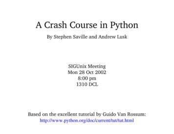
In [94]: def f(x): return x*np.cos(x**2)x np.linspace(-3,3,100)y f(x)plt.plot(x,y)Out[94]: [ matplotlib.lines.Line2D at 0x108783c18 ]We can plot more than one function by simply calling plt.plot multiple times. Here’s the graph of ftogether with is derivative.In [95]: def fp(x): return np.cos(x**2) - 2*x**2 * np.sin(x**2)yp fp(x)plt.plot(x,y)plt.plot(x,yp)Out[95]: [ matplotlib.lines.Line2D at 0x10875c860 ]17

There is much more that can be done with Matplotlib, as we’ll see throughout this book. Just this muchis very useful, however. Wouldn’t it be useful if we could have computed f 0 in the last example symbolically,though?2.3SymPySymPy is a rudimentary symbolic library for Python. I write “rudimentary” because, frankly, if you are usedto working with a commerical computer algebra system, like Mathematica or Maple, or even a good opensource tool, like Maxima, you might be disapointed in SymPy. It is simply much slower and less capablethan those tools. Nonetheless, it is can be convenient to have a tool for basic symbolic computation and itworks well with the other tools we are using for numerical computation. Other advantages of SymPy includethe fact that it is open source and can easily be used a library.SymPy is really not central to our needs; we will typ

A crash course in Python for elementary numerical computing January 10, 2016 This document was partly cobbled together byMark McClurefor his Math/CS 441 class in numerical computing atUNCA. It is largely based on a similar document byRick MullercalledA crash course in Python for Scientists- particularly, the extensive section entitled Python .