Transcription
6Fitting straight linesYou can go pretty far in data science using relatively simple visualand numerical summaries of data sets—tables, scatter plots, barplots, line graphs, boxplots, histograms, and so on. But in manycases we will want to go further, by fitting an explicit equation—usually called a regression model—that describes how one variablechanges as a function of some other variables. There are manyreasons we might want to do this. Here are three that we’ll explorein detail: to make a prediction; to summarize the trend in a data set; to make comparisons that adjust statistically for some systematic effect.This chapter introduces the idea of a regression model and buildsupon these themes.Fitting straight linesAs a running example we’ll use the data from Figure 6.1, whichdepicts a sample of 104 restaurants in the vicinity of downtownAustin, Texas. The horizontal axis shows the restaurant’s “fooddeliciousness” rating on a scale of 0 to 10, as judged by the writersof a popular guide book entitled Fearless Critic: Austin. The verticalaxis shows the typical price of a meal for one at that restaurant, including tax, tip, and drinks. The line superimposed on the scatterplot captures the overall “bottom-left to upper-right” trend in thedata, in the form of an equation: in this case, y 6.2 7.9x. Onaverage, it appears that people pay more for tastier food.This is our first of many data sets where the response (price,Y) and predictor (food score, X) can be described by a linearregression model. We write the model in two parts as “Y b 0 b 1 X error.” The first part, the function b 0 b 1 X, is calledthe fitted value: it’s what our equation “expects” Y to be, given X.
62data scienceFigure 6.1: Price versus reviewer foodrating for a sample of 104 restaurantsnear downtown Austin, Texas. Thedata are from a larger sample of 317restaurants from across greater Austin,but downtown-area restaurants werechosen to hold location relativelyconstant. Data from Austin FearlessCritic, www.fearlesscritic.com/austin. Because of ties in the data,a small vertical jitter was added forplotting purposes only. The equation ofthe line drawn here is y 6.2 7.9x.130120110100Price in Fearless Critic food ratingThe second part, the error, is a crucial part of the model, too, sinceno line will fit the data perfectly. In fact, we usually denote eachindividual noise term explicitly:y i b 0 b 1 x i ei .(6.1)Here the subscript i is just an index to denote which data pointwe’re talking about: i 1 for the first row of our data frame, i 9for the 9th, and so on.An equation like (6.1) is our first example of a regression model.The intercept b 0 and the slope b 1 are called the parameters of theregression model. They provide a mathematical description of howprice changes as a function of food score. The little ei is called theerror or the residual for the ith case—residual, because it’s howmuch the line misses the ith case by (in the vertical direction). Theresidual is also a fundamental part of the regression model: it’swhat’s “left over” in y after accounting for the contribution of x.For every two points. . . .A natural question is: how do we fit the parameters b 0 and b 1to the observed data? Historically, the standard approach, still inwidespread use today, is to use the method of least squares. Thisinvolves choosing b 0 and b 1 so that the sum of squared residuals
fitting straight lines6310108 C68 66810(the ei ’s) will be as small as possible. This is what we did to get theequation yi 6.2 7.9xi in Figure 6.1.The method of least squares is one of those ideas that, onceyou’ve encountered it, seems beautifully simple, almost to thepoint of being obvious. But it’s worth pausing to consider its historical origins, for it was far from obvious to a large number ofvery bright 18th-century scientists.To see the issue, consider the following three simple data sets.Each has only two observations, and therefore little controversyabout the best-fitting linear trend.B246810420200 A0244 02468100246810 b 0 1b 14 b 0 5b 188 b 0 7b 11036For every two points, a line. If life were always this simple, therewould be no need for statistics.But things are more complicated if we observe three points. CB3 b 0 1b 1 e14 b 0 5b 1 e28 b 0 7b 1 e3 .4 2 A0Two unknowns, three equations. There is no solution for the parameters b 0 and b 1 that satisfies all three equations—and thereforeno perfectly fitting linear trend exists. Seen graphically, at right, itis clear that no line can pass through all three points.Abstracting a bit, the key issue here is the following: how arewe to combine inconsistent observations? Any two points are consistent with a unique line. But three points usually won’t be, andmost interesting data sets have far more than three data points.Therefore, if we want to fit a line to the data anyway, we mustallow the line to miss by a little bit for each ( xi , yi ) pair. We express these small misses mathematically, as follows:0246810
1010data science1064ε3868 ε1246810 ε1 02 2 00ε2444 ε1 ε2ε202ε3 668ε3 0246810The three little e’s are the residuals, or misses.But now we’ve created a different predicament. Before weadded the ei ’s to give us some wiggle room, there was no solutionto our system of linear equations. Now we have three equationsand five unknowns: an intercept, a slope, and three residuals. Thissystem has infinitely many solutions. How are we to choose, forexample, among the three lines in Figure 6.2? When we changethe parameters of the line, we change the residuals, thereby redistributing the errors among the different points. How can this bedone sensibly?Believe it or not, scientists of the 1700’s struggled mightily withthis question. Many of the central scientific problems of this eraconcerned the combination of astronomical or geophysical observations. Astronomy in particular was a hugely important subjectfor the major naval powers of the day, since their ships all navigated usings maps, the stars, the sun, and the moon. Indeed, untilthe invention of a clock that would work on the deck of a shiprolling to and fro with the ocean’s waves, the most practical wayfor a ship’s navigator to establish his longitude was to use a lunar table. This table charted the position of the moon against the“fixed” heavens above, and could be used in a roundabout fashionto compute longitude. These lunar tables were compiled by fittingan equation to observations of the moon’s orbit.The same problem of fitting astronomical orbits arose in a widevariety of situations. Many proposals for actually fitting the equation to the data were floated, some by very eminent mathematicians. Leonhard Euler, for example, proposed a method for fittinglines to observations of Saturn and Jupiter that history largelyjudges to be a failure.0246810Figure 6.2: Three possible straightline fits, each involving an attemptto distribute the “errors” among theobservations.
fitting straight linesIn fact, some thinkers of this period disputed that it was evena good idea to combine observations at all. Their reasoning was,roughly, that the “bad” observations in your sample would corruptthe “good” ones, resulting in an inferior final answer. To borrowthe phrase of Stephen Stigler, an historian of statistics, the “deceptively simple concept” that combining observations would improveaccuracy, not compromise it, was very slow to catch on during theeighteenth century.1165The History of Statistics, p. 15.The method of least squaresNo standard method for fitting straight lines to data emerged untilthe early 1800’s, half a century after scientists first entertainedthe idea of combining observations. What changed things wasthe method of least squares, independently invented by two people.Legendre was the first person to publish the method, in 1805,although Gauss claimed to have been using it as early as 1794.The term “method of least squares” is a direct translation ofLegendre’s phrase “méthode des moindres carrés.” The idea issimple: choose the parameters of the regression line that minimizeÂin 1 ei2 , the sum of the squared residuals. As Legendre put it:In most investigations where the object is to deduce the mostaccurate possible results from observational measurements,we are led to a system of equations of the formE a bx cy f z &c.,in which a, b, c, f , &c. are known coefficients, varying fromone equation to the other, and x, y, z, &c. are unknown quantities, to be determined by the condition that each value of Eis reduced either to zero, or to a very small quantity. . . .Of all the principles that can be proposed for this purpose,I think there is none more general, more exact, or easier toapply, than that which we have used in this work; it consistsof making the sum of the squares of the errors a minimum. Bythis method, a kind of equilibrium is established among theerrors which, since it prevents the extremes from dominating,is appropriate for revealing the state of the system which mostnearly approaches the truth.2The utility of Legendre’s suggestion was immediately obvious to his fellow scientists and mathematicians. Very rapidly,least squares became the dominant method for fitting equationsthroughout the European scientific community.2Adrien-Marie Legendre (1805), Nouvelles méthodes pour la détermination desorbites des comètes. Translation p. 13,Stigler’s A History of Statistics.
66data scienceWhy was the principle adopted so quickly and comprehensively? For one thing, it offered the attractiveness of a single bestanswer, evaluated according to a specific, measurable criterion.This gave the procedure the appearance of objectivity—especiallycompared with previous proposals, many of which essentiallyamounted to: “muddle around with the residuals until you get anacceptable balance of errors among the points in your sample.”Moreover, unlike many previous proposals for combining observations, the least-squares criterion could actually be applied tonon-trivially large problems. One of the many advantages of theleast-squares idea is that it leads immediately from grand principleto specific instructions on how to compute the estimate ( bb0 , bb1 ):bb1bb0 Âin 1 ( xi x̄ )(yi ȳ)Âin 1 ( xi x̄ )2 ȳbb1 x̄ ,(6.2)(6.3)In statistics, a little hat on top of something usually denotes a guess or anestimate of the thing wearing the hat.where x̄ and ȳ are the sample means of the X and Y variables,respectively. The line y bb0 bb1 x is the best possible linear fit tothe data, in a squared-error sense. That is to say: among the familyof all possible straight-line fits to the data, this particular linehas the smallest sum of squared residuals. Deriving this solutioninvolves solving a simple mathematical problem involving somecalculus and matrix algebra. This is something that scientists ofthe nineteenth century could do via pen and paper—and that,happily, modern computers take care of for us nowadays.Goals of regression analysisThe estimation of linear regression models by least squares is nowentirely automatic using standard software for all but the verylargest of data sets.3 It’s so ordinary, in fact, that the method isoften abbreviated as OLS: ordinary least squares.But don’t let the simplicity of the model-fitting step fool you:regression modeling is a wonderfully rich and complex subject.We’ll start by focusing on four kinds of stories one can tell with aregression model. Each is useful for a different purpose.3By “very largest,” think: every searchthat Google has every recorded, everypost in the history of Facebook, and soforth. It’s still possible to fit regressionmodels to those data sets, but doing sois far from automatic—and possessingthe expertise necessary to do so is alarge part of what makes the major Silicon Valley companies so extraordinary(and so valuable).
fitting straight linesLeast squares then and now: an historical asideThe Ordnance Survey is the governmental body in the United Kingdom charged with mapping and surveying the British Isles. “Ordnance” is a curious name for a map-making body, but it has its roots in themilitary campaigns of the 1700’s. The name just stuck, despite the fact that these days, most of the folksthat use Ordnance Survey maps are hikers and bikers.In the days before satellites and computers, map-making was a grueling job, both on the soles of yourfeet and on the pads of your fingers. Cartographers basically walked and took notes, and walked and tooknotes, ad infinitum. In the 1819 survey, for example, the lead cartographer, Major Thomas Colby, endureda 22-day stretch where he walked 586 miles—that’s 28 miles per day, all in the name of precision cartography. Of course, that was just the walking. Then the surveyors would have to go back home and crunch thenumbers that allowed them to calculate a consistent set of elevations, so that they could correctly specifythe contours on their maps.They did the number-crunching, moreover, by hand. This is a task that would make most of us weep atthe drudgery. In the 1858 survey, for example, the main effort involved reducing an enormous mass ofelevation data to a system of 1554 linear equations involving 920 unknown variables, which the Ordnance Survey mathematicians solved using the principle of least squares. To crunch their numbers, theyhired two teams of dozens of human computers each, and had them work in duplicate to check each other’smistakes. It took them two and a half years to reach a solution.A cheap laptop computer bought today takes a second or less to solve the same problem.67
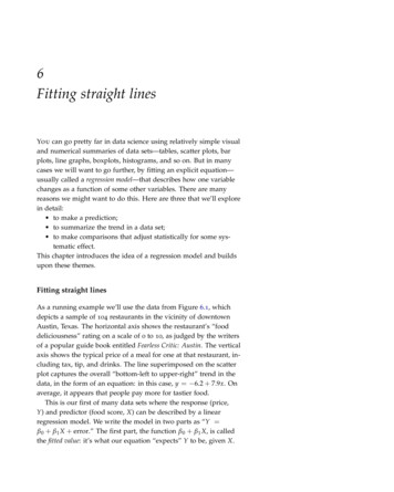
68data science8070Price (dollars/person)603) Go horizontally to the Y axis.Read off your prediction.502) Go verticallyup to the line.403020101) Start at the X whereyou want to predict.012345678910Austin Fearless Critic food ratingFigure 6.3: Using a regression modelfor plug-in prediction of the price of ameal, assuming a food rati
Figure 6.2: Three possible straight-line fits, each involving an attempt to distribute the “errors” among the observations. The three little e’s are the residuals, or misses. But now we’ve created a different predicament. Before we added the ei’s to give us some wiggle room, there was no solution to our system of linear equations .