Transcription
ARCHITECTING DATA MANAGEMENT:7 PRINCIPLES USING SAS , DATAFLUX AND SQLRobert P. Janka, Modern Analytics, San Diego, CAABSTRACTSeven principles frequently manifest themselves in data management projects. These principles improve twoaspects: the development process, allowing the programmer to deliver better code faster with fewer issues, and theactual performance of programs and jobs.Using examples from SAS(R) (Base / Macro), DataFlux(R) and SQL, this paper will present 7 principles, includingenvironments (e.g. DEV/TEST/PROD), job control data, test data, improvement, data locality, minimal passes, andindexing.Readers with an intermediate knowledge of SAS DataFlux Management Platform and/or Base SAS and SAS/Macroas well as SQL will understand these principles and find ways to utilize them in their data management projects.INTRODUCTIONDuring my current long-term consulting engagement for a financial services institution, which I will call “FINCO”, Irepeatedly encounter situations where one or more Data Management principles manifest. Many are these areessential in enterprise data management. The scale of work for Enterprise Data Management typically involves dailyupdates to tens or hundreds of tables, where we see daily data volumes in the range of 100,000 records all the wayup to 100 million records.In my experience, I find that these principles span all sorts of clients and companies. If a company is not yet operatingat the “enterprise” scale, its management probably hopes to reach that scale sometime in the not so distant future.Utilizing several of these principles will help the company better prepare for that future.Some key motivations for these principles are improvements in quality, delivery times, and/or performance of the datamanagement projects. These principles are not an exclusive list, but represent some of the more common datamanagement principles.Many of these principles are present in some aspect of SAS Data Integration Studio and/or DataFlux DataManagement Platform. Although these platforms are typically used by companies that need Enterprise DataManagement solutions, this paper will present illustrative examples that use only Base SAS , including SAS Macroand PROC SQL.OVERVIEW OF DATAFLUX DATA QUALITY (DQ) PROCESS AND DQMARTAt “FINCO”, I and several other team members design, develop and maintain the technology portions of a DataQuality process using DataFlux Data Management Platform (DMP). Another team, the Data Management staff, workwith the Data Stewards in the Lines of Business to identify Key Business Elements (KBE), profile those fields, anddevelop business rules to ensure data quality in those fields.To profile a KBE field, the Data Steward will sample the data for a few business DATE ID values and determineseveral key aspects: missing counts (aka how many NULL values), data type (character, numeric, date, etc.), andfrequency counts. Most SAS programmers will notice that this mirrors the mantra “Know Thy Data”. Let me repeat,“Know Thy Data”.After profiling the KBE fields, the Data Steward then writes English version of the Business Rules. For one KBE, thebusiness rule might be as simple as “Field X cannot be NULL or empty”. For another KBE, the rule might be this:“Field Y must be one of these values: Past Due, Current, Paid Off”. The Data Management staff then develop theDataFlux version of each business rule using the DataFlux Expression Engine Language.Our DataFlux process jobs then run a collection of business rules, grouped into a DataFlux data job, on the specifiedtable and business DATE ID. DataFlux moves data differently than SAS: The data input node reads 1 record at atime and passes it to the next node in the job. In the Monitor Node, each of the appropriate business rules run ontheir respective fields in the record. If a business rule “fails”, then the Monitor data job writes certain portions of therecord, usually including the business rule field and any pass-through fields, such as unique identifier, grouping fields,and/or balance fields, to the DataFlux repository as a “trigger” record. After the monitor phase completes, the Reportphase extracts the “trigger” records, and generates 2 result tables: one with each failed record (DETAILS) and onePage 16 September 2015
which aggregates the records (SUMMARY). The summary table adds up the balance fields, grouped by rule field andthe grouping fields.On the other hand, each SAS step (DATA or PROC) reads *all* input records, processes all of them, and then writesall output records.“FINCO” is definitely at the Enterprise Data Management level, with over 50 source tables updated daily. Many havedata volumes less than 10000 records while some have well over 1 million records processed every day. My fellowDQ technology team members and I have developed a small number of DataFlux process job streams which enableus to quickly add a new source table without changing any code in the process jobs.NOTES:Throughout this paper, I advocate a process of examine, hypothesize, test, and act. Examine your code for potential improvements.Hypothesize an improvement.Try out the improvement.If it yields the desired results, implement it. If not, then restart at Examine.ENVIRONMENTS PRINCIPLE:USE SEPARATE ENVIRONMENTS IN SEQUENCE TO DEVELOP AND TEST CODE,AND THEN TO GENERATE PRODUCTION RESULTS.BENEFIT:FIND AND RESOLVE PROBLEMS *BEFORE* WE PUT CHANGES INTO PRODUCTION USE.Like many larger companies, “FINCO” has three shared environments: DEV, TEST, and PROD. Each environmentaccesses different databases for the source and results data. The source data usually points to the ETL environmentat the same level. Thus, as the ETL developers add a new table at their DEV database, we can point our DataFluxjobs at DEV to read that new table.DataFlux developers use local environments on their workstations to develop process and data jobs independent ofeach other. They then ‘check-in’ or commit these changes to a versioning control system, i.e. Subversion. At eachshared environment in succession, they coordinate changes in the environment using “check-out” or “update”.Other version control systems include RCS, CVS, Git, and Visual SourceSafe. Two main benefits derive from use ofversion control systems. First, we can quickly revert to a previous version that is known to work if we ever commitchanges that have an unexpected issue not caught during development or testing. Second, we can compare twoversions to see what actual changes are present in the two versions, along with any explanatory notes included withthose changes. A very frequent example is the comparison of a new set of changes to the current shared version. Ifthe developer only sees the expected changes, then she has a higher confidence that her new changes will not breakany existing functionality.We leverage the macro variable facility in DataFlux to set some common values on a per-environment basis. Thisallows us to easily promote a job from one environment to the next, knowing that it will configure itself to use thecorresponding source and target data locations. In DataFlux, we use 3 common values: Environmento %%DF ENV%%Source DataSourceName (DSN)o %%SRC DSN%%Destination DataSourceName (DSN)o %%DEST DSN%%In Base SAS, we can emulate these variables by using the SAS Macro facility. For example, I wrote a very simplemacro called %LOAD ENV() that takes an optional Level Env parameter. If no parameter is specified, then itdefaults to “DEV”.Page 26 September 2015
The readers can try this out for themselves by specifying a different “autoexec.sas” script when they invoke SAS. Forexample, you might have an “autoexec dev.sas” for the DEV environment and an “autoexec tst.sas” for the TESTenvironment. In the “autoexec ENV.sas” file, call the %LOAD ENV() macro with the specified level env value (“DEV”in “autoexec dev.sas” and “TST” in “autoexec tst.sas”)./** SAS Macro:** Purpose:environments.** Author:* Date:**/load env()Demonstrate how to load macro variables for DEV, TEST, PRODBob Janka2015-07%macro load env(env level DEV);/** %let var path "C:\SAS\&env level\env vars.sas";*/%globalSRC DSNDEST DSNMETA DSN;%IF &env level DEV %then %DO;%let SRC DSN DEV SRC;%let DEST DSN DEV DEST;libnamelibname%END;&SRC DSN.&DEST DSN.base "C:\SAS\&env level\data src";base "C:\SAS\&env level\data dest";%ELSE %IF &env level TST %then %DO;%let SRC DSN TST SRC;%let DEST DSN TST DEST;libnamelibname%END;&SRC DSN.&DEST DSN.%ELSE %DO;%put load env:%END;base "C:\SAS\&env level\data src";base "C:\SAS\&env level\data dest";Unknown environment level: "&env level";%MEND;options mprint;%load env(env level DEV);***%load env(env level TST);%load env(env level BAR);%load env();Log of above SAS program is shown here:50%load env(env level DEV);MPRINT(LOAD ENV):libname DEV SRC base "C:\SAS\DEV\data src";NOTE: Libref DEV SRC was successfully assigned as follows:Engine:BASEPhysical Name: C:\SAS\DEV\data srcPage 36 September 2015
MPRINT(LOAD ENV):libname DEV DEST base "C:\SAS\DEV\data dest";NOTE: Libref DEV DEST was successfully assigned as follows:Engine:BASEPhysical Name: C:\SAS\DEV\data destBase SAS provides a system option, SYSPARM, that allows us to specify an environment value for a set ofprograms. If we need to specify multiple different values in the SYSPARM option, we could introduce separatorcharacters, such as a colon (:), and then write a macro to parse out the different strings and assign those to knownglobal macro variables for use by later macros and modules.The specifics are less important than the concept: use macro variables to set per-environment values that allow youto point your job or program to different input data and save the results in separate locations.JOB CONTROL PRINCIPLE:USE INTERNAL CONTROL TABLE IN DATABASE TO CONTROL JOB RUNS.BENEFIT:RE-USE CODE FOR MULTIPLE SETS OF ROUGHLY SIMILAR INPUT DATA.Job control tables provide the capability to run the same job or program with different inputs and track those individualruns. Using a job control table enables us to write the job once and then re-use it for each new source table. If youput any table-specific processing into the monitor data job, then for each new source table, you need only do thefollowing: Create table-specific monitor data jobo This runs the business rules for that specific table. Each table gets its own monitor data job.Add 1 record to control table, DF META TABLESAdd k records to control table, DF META FIELDS,o Where k is the number of rule fields PLUS the number of pass-through fields.o Each record in this control table specifies one of these fields.We have 2 control tables: one that manages control data for each source table (DF META TABLES) and anotherthat manages control data for each KBE field in those source tables (DF META FIELDS). We configure our jobs totake 2 job-level parameters: a source table name and a business DATE ID. The job looks up the source table namein our control table, DF META TABLES, extracts the table-specified metadata, and then starts processing thatsource table.The job has 3 phases: a Count phase, a Monitor phase, and a Report phase. The Count phase submits a query tothe source table that does a simple count, filtering on only those records with the specified business DATE ID. Formost source tables, we expect data on a daily basis. If the count is zero, then the job quits with an error message.For the Monitor phase, the job queries the control table, DF META FIELDS, to get a list of the fields for the specifiedsource table. The job then invokes the table-specific data job to run the business rules for that source table. Eachthread builds up a query to the source table, using the list of source fields and a filter on the business DATE ID.In the Report phase, the job uses the table-specific information from the control table, DF META TABLES, todetermine which source fields to use for the Balance and grouping fields. It then submits another query to the sourcetable to aggregate the day’s data by the grouping fields and summing up the Balance field. These aggregated recordsprovide the TOTAL record counts and TOTAL balances, by grouping variable, for the day’s source data. It nextextracts the trigger records from the DataFlux repository. Each of these records, including the Unique ID field, arewritten to the results table, DQ DETAIL. These records provide an exact list of which source records failed whichbusiness rules and the values that caused these failures. The same trigger records are summarized by groupingvariable and then combined with the TOTAL counts and balances to populate the results table, DQ SUMMARY.In the SAS code shown below, it first creates the control tables and populates them with some example control data.It then shows some lookups of these control data. In the second control table, DF META FIELDS, thePage 46 September 2015
SQL FIELD EXPRSSN usually contains a simple expression, consisting solely of the source field name. It couldcontain a more complex expression that combines multiple source fields into a single composite monitor field. Theexample shows a numeric expression that adds two source fields to yield an amount field.SAS program shown here:/** Job Control Data - Setup*/%load env();/*DQMart – DF META TABLESdata &DEST DSN.DF META TABLES;attrib PRODUCT GROUP lengthattrib SRC TABLElengthattrib SRC CATEGORYlengthattrib SRC AMOUNTlength*/ 10; 20; 10; 20;INPUT PRODUCT GROUP SRC TABLE SRC CATEGORY SRC AMOUNT;DATALINES;/* aka CARDS; */LOANSBUSINESS LOANSREGION BUSINESS BALANCELOANSPERSONAL LOANSBRANCH PERSONAL BALANCEDEPOSITS ACCOUNTSCHK SAV NET BALANCE;PROC PRINT data &DEST DSN.DF META TABLES;run;/*DQMart – DF META FIELDSdata &DEST DSN.DF META FIELDS;attrib PRODUCT GROUPlengthattrib SRC TABLElengthattrib TECH FIELDlengthattrib SQL FIELD EXPRSN length*/ 10; 20; 10; 200;INPUT PRODUCT GROUP 1-10 SRC TABLE 11-30 TECH FIELD 31-40SQL FIELD EXPRSN & 41-101;DATALINES;/* aka CARDS; */LOANSBUSINESS LOANSREGIONREGIONLOANSBUSINESS LOANSBALANCECoalesce(Principal,0) Coalesce(Interest,0) as PERSONAL BALANCELOANSBUSINESS LOANSField1Field1LOANSBUSINESS LOANSField2Field2;/* NOTE: 2nd and 3rd datalines above are actually all one line */PROC PRINT data &DEST DSN.DF META FIELDS;run;/** Job Control Data - Usage*//**Page 5Get fields to process for source table6 September 2015
*/proc sql noprint;selectSQL FIELD EXPRSNinto:SRC FIELDS SEPARATED by " , "from &DEST DSN.DF META FIELDSwhereSRC TABLE 'BUSINESS LOANS'order byTECH FIELD;quit;%PUT&SRC FIELDS;%LET%LET%LET%LETsql text 00sql text 01sql text 02sql text 03 select ; from &SRC DSN.&SRC TBL ; where ; date var '20150704' ;%put%put%put%put&sql text 00&sql text 01&sql text 02&sql text 03;;;;%LET sql text flds &sql text 00&SRC FIELDS&sql text 01&sql text 02&sql text 03;%put &sql text flds ;SAS listing output from above program shown here:The SAS S4LOANSSRC TABLE16:08 Monday, July 13, 2015TECHFIELDBUSINESS LOANS REGIONBUSINESS LOANS BALANCEas PERSONAL BALANCEBUSINESS LOANS Field1BUSINESS LOANS Field21SQL FIELD EXPRSNREGIONCoalesce(Principal,0) CoalesceField1Field2SAS log output from above program shown here:92939495Page 6/** Get fields to process for source table*/6 September 2015
96proc sql noprint;97select98SQL FIELD EXPRSN99into100:SRC FIELDS SEPARATED by " , "101from &DEST DSN.DF META FIELDS102where103SRC TABLE 'BUSINESS LOANS'104order by105TECH FIELD106;NOTE: The query as specified involves ordering by an item that doesn'tappear in its SELECTclause.107 quit;NOTE: PROCEDURE SQL used (Total process time):real time0.06 secondscpu time0.01 seconds108109%PUT&SRC FIELDS;coalesce(Principal,0) coalesce(Interest,0) as PERSONAL BALANCE , Field1, Field2 , REGION112 %LET sql text 00 select ;113 %LET sql text 01 from &SRC DSN.&SRC TBL ;114 %LET sql text 02 where ;115 %LET sql text 03 date var '20150704' ;116126 %put &sql text 00 ;select127 %put &sql text 01 ;from DEV SRC.BUSINESS LOANS128 %put &sql text 02 ;where129 %put &sql text 03 ;date var '20150704'132133134135136137138139140%LET sql text flds &sql text 00&SRC FIELDS&sql text 01&sql text 02&sql text 03;%put &sql text flds ;selectcoalesce(Principal,0) coalesce(Interest,0) as PERSONAL BALANCE, Field1 , Field2 , REGIONfrom DEV SRC.BUSINESS LOANSwheredate var '20150704'Page 76 September 2015
TEST DATA PRINCIPLE:ADD SUPPORT TO REDIRECT SOURCE AND/OR TARGET DATA FOR TESTING.BENEFIT:USE DIFFERENT SETS OF TEST OR SAMPLE DATA WHEN TESTING PROGRAMS ORJOBS.Before we can explore performance improvements, we need to know that the DataFlux jobs and SAS programs arebehaving correctly. Make them do the “right” things *before* you try to speed them up!In the previous principle of Environments, we set some environment defaults. In this principle, we extend our jobs andprograms to allow run-time changes that override those defaults.Many jobs and programs read data from a source, process that data, and then write out results to a destination. OurDataFlux jobs at “FINCO” do this also. We add a node at the beginning of the job that reads 2 key job-levelparameters: SRC DSN and DEST DSN (where DSN is DataSourceName, which anyone familiar with ODBC willprobably recognize).The job looks for override values at run-time. If no values are provided, then the job looks up the default values in theenvironment settings.We also added another job-level parameter: TABLE PREFIX. If not provided, we detect the default value and set thejob-level parameter to NULL. If it is provided, then we set the job-level parameter to its value. Our table referencesnow look this in SAS (periods are necessary to terminate SAS macro variable references in text strings):&SRC DSN.&TABLE PREFIX.&TABLE NAME.For “FINCO”, some of the rule fields never have any “bad” data in the live source tables. How can we show that therule logic works for these fields? By creating an alternate set of source tables with test data. When we create this testdata, we want to include both “good” data and “bad” data. For many rules, the logic is fairly simple: “The rule fieldmust NOT be NULL or blank”. We can sample one record from the live source table as our “good” data. We can thencopy that record and set the values for the various rule fields in that table to NULL. This should yield 1 “FAILED” and1 “PASSED” instance for each rule on that table. If the logic uses something else, like this:“The rule fieldmust be numeric and not zero”, we can set the “bad” data to a zero (0). In any case, we want to force each rule to“pass” at least 1 record and “fail” at least 1 record. For some tables, we had several test records to cover morecomplex rule logic.Where do we put the test data? At “FINCO”, we do not have write access to the source database. So, we create thetest tables in our DQMart schema and use a table prefix of “TD ”. This allows us to separate out test data fromsample data “SD ” which we used to help develop rule logic for some other source tables.One advantage to using test or sample data is that these runs will complete a LOT faster with 10-100 recordscompared to some live source tables which yield over 100,000 records on a daily basis.An associated suggestion in this principle involves the logging of any SQL queries generated by the job or programand submitted to the source database. SAS programmers are lucky in that PROC SQL usually writes to the SAS logthe query it submits to the database. If you are encountering issues with the submitted queries in SAS, you canextract the exact SQL query text from the log and submit in a database client, which eliminates any SAS overhead orissues from your troubleshooting. These external client submissions often yield more detailed error messages thathelp the developer pinpoint the problem in the query.In DataFlux, we build up text blocks containing the generated SQL queries and then submit those in the job. Weadded a few statements to write out those blocks to the job log which enable our troubleshooting.SAS program shown here:/** Test Data - Setup*/data &DEST DSN.TD LOAN;attrib Field XPage 8length 4;6 September 2015
attribattribattribINPUTField YExpect XExpect YField XDATALINES.9;01/*failpasslength 4;length 8;length 8;Field YExpect Xaka CARDS;Expect Y;*/;failpassproc print data &DEST DSN.TD LOAN;run;/** Test Data - Usage*/%put ;%let table prefix ;%put Data &dest dsn.&table prefix.&src tbl;%put ;%let table prefix TD ;%put Data &dest dsn.&table prefix.&src tbl;%put ;%let table prefix SD ;%put Data &dest dsn.&table prefix.&src tbl;SAS listing output from above program shown here:ObsField XField YExpect XExpect Y12.901failpassfailpassSAS log output from above program shown here:323324proc print data &DEST DSN.TD LOAN;run;NOTE: There were 2 observations read from the data set DEV DEST.TD LOAN.NOTE: PROCEDURE PRINT used (Total process time):real time0.01 secondscpu time0.01 seconds333334Data335336337Data338Page 9%let table prefix ;%put Data &dest dsn.&table prefix.&src tbl; DEV DEST.BUSINESS LOANS%let table prefix TD ;%put Data &dest dsn.&table prefix.&src tbl; DEV DEST.TD BUSINESS LOANS6 September 2015
339340Data341%let table prefix SD ;%put Data &dest dsn.&table prefix.&src tbl; DEV DEST.SD BUSINESS LOANS%put ;IMPROVEMENT PRINCIPLE:USE THE PARETO PRINCIPLE (20/80 RULE) REPEATEDLY AS NEEDED.oStay alert for opportunities to improve Improvements can be in the code Improvements can also be in the development processBENEFIT:FOCUS IMPROVEMENT EFFORTS ON MOST SIGNIFICANT FACTORS.The first three principles focus on the development process while the last three principles focus on the performanceof programs and jobs.In our development, we start with “good enough” code that meets the minimum quality and performancerequirements. Over time, as we modify the code to add some of the inevitable changes required with new source datathat has different needs, we strive to improve both the quality and performance.We now expand our focus to a broader topic, that of continual improvement. When we have an opportunity to reviewthe existing code base for jobs or programs, we want to take a few minutes and see if there are any improvementsthat we might have identified during production runs. Perhaps our jobs are taking longer amounts of time to complete.Often times, we have pressures to deliver jobs or programs by a particular deadline. This forces us to choose whatitems we have to do before the deadline and which items can wait for a future change opportunity. If we keep theseitems in a list somewhere, then the next time we are making changes to the job or program, we can review them forinclusion.Use the 20/80 rule: where 20% of factors explain (or yield) 80% of results. One way to view this is that we can usuallyfind a few items to improve for now and leave others for later. Another thing to keep in mind is that we don’t have tofix *everything* *all of the time*. Often, we get “good enough” results by resolving a few critical items.ooFind the one or few factors that explain a majority of the issues.Resolve these and observe the results.To help us focus on the key aspects of our computations, let me introduce a concept from Computer Science, namelyOrder Notation (aka Big-O Notation). This notation helps us compare algorithms and even full programs by assessingcosts involved in getting data, processing it, and saving the results.The full details of Order Notation are beyond the scope of this paper, but we can get a general sense of somecommon cost assessments. There are 4 common examples: O( N )o Linear time to perform operations.O( logN )o Logarithmic time to perform operationsO( N * logN )o N* Logarithmic time to perform operations.O( N * N )o Quadratic time to perform operations.Each of these examples assess the costs of performing a particular set of operations based on the number of itemsgoing those operations. For instance, when N 10, the differences are fairly small between Linear and Logarithmic.When N exceeds one thousand ( 1 000 ) or one million ( 1 000 000 ), then the differences are quite dramatic.P a g e 106 September 2015
Here is a graph where N varies from 10 to 100 by 10, including the O( N * N ) case.Since the O( N * N) increases greatly with larger values for N, this squeezes together the other 3 Order Notationexpressions. To help clarify their relative increases, I show a second graph without the O( N * N ) values.Here is a graph where N varies from 10 to 100 by 10, excluding the O( N * N ) case.P a g e 116 September 2015
Why do we want to use Order Notation? A key teaching example is the difference between efficient and inefficientsorting algorithms. Many efficient sorting algorithms perform in N* logarithmic time at O( N * logN ). These includealgorithms such as quicksort and mergesort. Inefficient sorting algorithms, such as insertion sort and bubble sort,tend to perform in quadratic time at O( N * N ).Binary searches or heap operations are a common example of logarithmic time at O( logN ).What is a key learning from Order Notation? The costs of certain classes of operations are more expensive thanothers. Data Management professionals should strive to reduce these classes, which are most likely sorts. Althoughwe cannot eliminate them entirely, we have several strategies to consider: Combine multiple sorts into a single sort.Defer sorting until after data is pruned.Sort keys to the data instead of the data itself.As we explore the next few Data Management principles, I will refer to the corresponding Order notations.For SAS programmers, I strongly encourage to set option FULLSTIMER. This gives you details on how much CPUand I/O is used for each DATA or PROC step. If you extract these details with the name of the PROC or DATA step,then you sort these details to find which steps consume the most amount of time in your program. If you want toassess the Order Notation for your program, try running multiple tests with different scales of observations, say 10,100, 1000. You can then plot your total time to see which curve approximates the run-times.P a g e 126 September 2015
DATA LOCALITY PRINCIPLE:MOVE COMPUTATIONS AS CLOSE AS POSSIBLE TO DATA.BENEFIT:IMPROVE PERFORMANCE BY REDUCING DATA TRANSFER TIMESIn many Enterprise Data Management environments, data moves between multiple database and compute server.This introduces overhead in moving data across a network, which is usually 10-1000 times slower than moving datainternally in a server. Efficient data management dictates that we process the data as close to the source as possibleto reduce the network overhead.One example for data locality is pushing computations into the database, especially any summarizations and/oraggregations. If we look at the effort required to pull data from a source database into SAS, then run PROCsummary, and then save results, we can use this Order Notation expression:T k * O( N ) Summary( N ) k * O( M )where:k is a constant factor representing the overhead of moving data over the network.N is the number of source recordsM is the number of result records.Summary( N ) is the time to run PROC SUMMARY.If we are summarizing to a much smaller number of result records, then it is more efficient to move thatsummarization to the database as much as possible. Here is an example using a common SQL concept ofsubqueries:/****/Data Locality Principleproc sql;selectSQ.count rows,SQ.sum actual,SQ.prodtype,SQ.product,(SQ.sum actual / SQ.count rows )from (selectcount( * ) as count rows,sum(actual) as sum actual,prodtype,productfrom sashelp.prdsal2group byprodtype,product) SQ;quit;asAvg salesOur new Order Notation expression would now look like this:T Summary( N ) k * O( M )Where we have eliminated the first factor of “k * O(N)”.Summary( N ) is the time to run the SQL summarization query(assumption: PROC SUMMARY and SQL summarization query take roughly the same amount of time).P a g e 136 September 2015
In DataFlux, all SQL queries are passed directly to the source database. In Base SAS, PROC SQL has two modes:implicit pass-through and explicit pass-through. The mode is determined by how you connect to the database. If youcreate a libname and then use SAS libname.dataset notation in your SQL query, PROC SQL will implicitly pass thequery pieces to the source database via a SQL query translator. If you use a connect statement, then PROC SQLdirectly connects to the source database in “explicit” mode. For many queries which use generic SQL expressions,there should be little difference. If you find that you need a database-specific function or expression, then you mustuse the connect() statement and “explicit” mode. Be aware that this code now locks into the SQL dialect of thatsource database. If you try to change databases, say from Oracle to Netezza or SQL Server to Teradata, then youwill have to review these queries and possibly rewrite them to work with the new dialect.SAS listing output from above program shown here:count rowssum DSOFACHAIRDESKAvg sales644.1409674.3382641.5597645.5484SAS log output from above program shown here:230 proc sql;231select232SQ.count rows233,SQ.sum actual234,SQ.prodtype235,SQ.product236,(SQ.sum actual / SQ.count rows ) as237from (238select239count( * ) as count rows240,sum(actual) as sum actual241,prodtype242,product243from sashelp.prdsal2244group by245prodtype246,product247) SQ248;249 quit;NOTE: PROCEDURE SQL used (Total process time):real time0.03 secondscpu time0.03 secondsP a g e 14Avg sales6 September 2015
MINIMAL PASSES PRINCIPLE:TOUCH EACH OBSERVATION / RECORD AS FEW TIMES AS POSSIBLE.BENEFIT:IMPROVE PERFORMANCE BY REDUCING MULTIPLE READS OF DATA.The principle of Minimal Passes is similar to Data Locality, but deals more wi
Many of these principles are present in some aspect of SAS Data Integration Studio and/or DataFlux Data Management Platform. Although these platforms are typically used by companies that need Enterprise Data Management solutions, this paper will present illustrative examples that use only Base SAS , including SAS Macro and PROC SQL.


![Academy Cloud Foundations Course Outline [English]](/img/13/academy-20cloud-20foundations-20course-20outline-20-english.jpg)