Transcription
Chapter 1Review of Energy DispersionRelations in SolidsReferences: Ashcroft and Mermin, Solid State Physics, Holt, Rinehart and Winston, 1976, Chapters 8, 9, 10, 11. Bassani and Parravicini, Electronic States and Optical Transitions in Solids, Pergamon, 1975, Chapter 3. Kittel, Introduction to Solid State Physics, Wiley, 1986, pp. 228-239. Mott & Jones – The Theory of the Properties of Metals and Alloys, Dover, 1958 pp.56–85. Omar, Elementary Solid State Physics, Addison–Wesley, 1975, pp. 189–210. Ziman, Principles of the Theory of Solids, Cambridge, 1972, Chapter 3.1.1IntroductionThe transport properties of solids are closely related to the energy dispersion relations E( k)in these materials and in particular to the behavior of E( k) near the Fermi level. Conversely, the analysis of transport measurements provides a great deal of information onE( k). Although transport measurements do not generally provide the most sensitive toolfor studying E( k), such measurements are fundamental to solid state physics because theycan be carried out on nearly all materials and therefore provide a valuable tool for characterizing materials. To provide the necessary background for the discussion of transportproperties, we give here a brief review of the energy dispersion relations E( k) in solids. Inthis connection, we consider in Chapter 1 the two limiting cases of weak and tight binding.In Chapter 2 we will discuss E( k) for real solids including prototype metals, semiconductors,semimetals and insulators.1
1.21.2.1One Electron E( k) in SolidsWeak Binding or Nearly Free Electron ApproximationIn the weak binding approximation, we assume that the periodic potential V ( r) V ( r R n )is sufficiently weak so that the electrons behave almost as if they were free and the effectof the periodic potential can be handled in perturbation theory (see Appendix A). In thisformulation V ( r) can be an arbitrary periodic potential. The weak binding approximationhas achieved some success in describing the valence electrons in metals. For the core electrons, however, the potential energy is comparable with the kinetic energy so that coreelectrons are tightly bound and the weak binding approximation is not applicable. In theweak binding approximation we solve the Schrödinger equation in the limit of a very weakperiodic potentialHψ Eψ.(1.1)Using time–independent perturbation theory (see Appendix A) we writeE( k) E (0) ( k) E (1) ( k) E (2) ( k) .(1.2)and take the unperturbed solution to correspond to V ( r) 0 so that E (0) ( k) is the planewave solutionh̄2 k 2E (0) ( k) .(1.3)2mThe corresponding normalized eigenfunctions are the plane wave states(0)ψ ( r)k eik· r 1/2Ω(1.4)in which Ω is the volume of the crystal.The first order correction to the energy E (1) ( k) is the diagonal matrix element of theperturbation potential taken between the unperturbed states:(0)(0)E (1) ( k) hψ V ( r) ψ i kR Ω10 Ω0 Vk( r)d3 r1 R i k· rVΩ Ωe ( r)eik· r d3 r(1.5) V ( r)where V ( r) is independent of k, and Ω0 is the volume of the unit cell. Thus, in first orderperturbation theory, we merely add a constant energy V ( r) to the free particle energy, andthat constant term is exactly the mean potential energy seen by the electron, averaged overthe unit cell. The terms of interest arise in second order perturbation theory and are0X h k 0 V ( r) ki 2(1.6)E (2) ( k) (0) ( k) E (0) ( k 0 ) k0 Ewhere the prime on the summation indicates that k 0 6 k. We next compute the matrixelement h k 0 V ( r) ki as follows:R (0) (0)h k 0 V ( r) ki Ω ψ 0 V ( r)ψ d3 rk Ω1 Ω1RΩeRΩe2k i( k0 k)· rVi q · rV( r)d3 r( r)d3 r(1.7)
where q is the difference wave vector q k k 0 and the integration is over the whole crystal. n where r 0 is an arbitrary vector inWe now exploit the periodicity of V ( r). Let r r 0 R n is a lattice vector. Then because of the periodicity V ( r) V ( r 0 )a unit cell and RZ1Xh k 0 V ( r) ki Ω n 0 eiq·( r Rn ) V ( r 0 )d3 r0(1.8)Ω0where the sum is over unit cells and the integration is over the volume of one unit cell.ThenZ1 X iq· n0 R 0 eeiq· r0 V ( r 0 )d3 r .(1.9)hk V ( r) ki Ω nΩ0 n and for the wave vector qWriting the following expressions for the lattice vectors R n P3 nj ajRj 1 q where nj is an integer, then the lattice sumXe n Riq·n (1.10) j 1 αj bjP3"Pne n Riq·can be carried out exactly to yield3Y1 e2πiNj αjj 11 e2πiαj#(1.11)where N N1 N2 N3 is the total number of unit cells in the crystal and αj is a real number.This sum fluctuates wildly as q varies and averages to zero. The sum is appreciable only if q 3Xmj bj(1.12)j 1where mj is an integer and bj is a primitive vector in reciprocal space, so that q must be areciprocal lattice vector. Hence we haveXn ei q·Rn N δq ,G (1.13) n 2πljn where ljn is an integer.since bj · R This discussion shows that the matrix element h k 0 V ( r) ki is only important when q G0is a reciprocal lattice vector k k from which we conclude that the periodic potentialV ( r) only connects wave vectors k and k 0 separated by a reciprocal lattice vector. We notethat this is the same relation that determines the Brillouin zone boundary. The matrixelement is thenZN 00 hk V ( r) ki eiG· r V ( r 0 )d3 r 0 δ k0 k,G (1.14)ΩΩ0whereN1 (1.15)ΩΩ0and the integration is over the unit cell. We introduce VG Fourier coefficient of V ( r)whereZ1 0eiG· r V ( r 0 )d3 r 0(1.16)VG Ω0Ω03
so thath k 0 V ( r) ki δ k k0 ,G VG .(1.17)We can now use this matrix element to calculate the 2nd order change in the energy basedon perturbation theory (see Appendix A)E(2)( k) X GÃ VG 22m202k (k )h̄2! VG 22m X. k)2h̄2 k 2 (G(1.18)G k)2 the denominator in Eq. 1.18 vanishes and E (2) ( k) canWe observe that when k 2 (Gbecome very large. This condition is identical with the Laue diffraction condition. Thus,at a Brillouin zone boundary, the weak perturbing potential has a very large effect andtherefore non–degenerate perturbation theory will not work in this case.For k values near a Brillouin zone boundary, we must then use degenerate perturbationtheory (see Appendix A). Since the matrix elements coupling the plane wave states k and k G do not vanish, first-order degenerate perturbation theory is sufficient and leads tothe determinantal equationin which (0) E (k) E (1) ( k) E h k V ( r) k Gi ( r) kih k G V 0 (0)(1) E (k G) E (k G) E (1.19)2 2kE (0) ( k) h̄2m(1.20)E (0) ( kand 2 2 h̄ ( k G)G) 2mE (1) ( k) h k V ( r) ki V ( r) V0(1.21)E (1) ( k k G V ( r) k Gi V0 . G) hSolution of this determinantal equation (Eq. 1.19) yields: V 2 0,[E V0 E (0) ( k)][E V0 E (0) ( k G)]G(1.22)or equivalently [V0 E (0) ( k)][V0 E (0) ( k G)] V 2 0. (1.23)E 2 E[2V0 E (0) ( k) E (0) ( k G)]GSolution of the quadratic equation (Eq. 1.23) yields1 E V0 [E (0) ( k) E (0) ( k G)]2 r1 (0) 2 V 2[E (k) E (0) ( k G)]G4(1.24)and we come out with two solutions for the two strongly coupled states. It is of interest tolook at these two solutions in two limiting cases:4
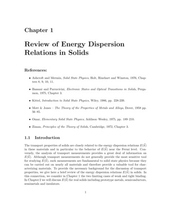
case (i) VG ¿ 12 [E (0) ( k) E (0) ( k G)] In this case we can expand the square root expression in Eq. 1.24 for small VG toobtain: E( k) V0 12 [E (0) ( k) E (0) ( k G)] 12 [E (0) ( k) E (0) ( k · [1 G)]22 VG 2[E (0) ( k) E (0) ( k G)](1.25) . . .]which simplifies to the two solutions:E ( k) V0 E (0) ( k) VG 2 E (0) ( k) E (0) ( k G) E ( k) V0 E (0) ( k G) VG 2 E (0) ( k)E (0) ( k G)(1.26)(1.27)and we recover the result Eq. 1.18 obtained before using non–degenerate perturbationtheory. This result in Eq. 1.18 is valid far from the Brillouin zone boundary, but nearthe zone boundary the more complete expression of Eq. 1.24 must be used. case (ii) VG À 12 [E (0) ( k) E (0) ( k G)] Sufficiently close to the Brillouin zone boundary ¿ V E (0) ( k) E (0) ( k G) G(1.28)so that we can expand E( k) as given by Eq. 1.24 to obtain· 21 (0) 1 [E (0) ( k) E (0) ( k G)](0) E (k) [E (k) E (k G)] V0 VG . (1.29)28 VG 1 V0 V , [E (0) ( k) E (0) ( k G)]G2(1.30)so that at the Brillouin zone boundary E ( k) is elevated by VG , while E ( k) is is the reciprocaldepressed by VG and the band gap that is formed is 2 VG , where G andlattice vector for which E( kB.Z. ) E( kB.Z. G)VG 1Ω0Z eiG· r V ( r)d3 r.(1.31)Ω0From this discussion it is clear that every Fourier component of the periodic potentialgives rise to a specific band gap. We see further that the band gap represents a range ofenergy values for which there is no solution to the eigenvalue problem of Eq. 1.19 for real k(see Fig. 1.1). In the band gap we assign an imaginary value to the wave vector which canbe interpreted as a highly damped and non–propagating wave.5
Figure 1.1: One dimensional electron energy bands for the nearly free electron model shownin the extended Brillouin zone scheme. The dashed curve corresponds to the case of freeelectrons and the solid curves to the case where a weak periodic potential is present. Theband gaps at the zone boundaries are 2 VG . the smaller the value of V , so that higherWe note that the larger the value of G,GFourier components give rise to smaller band gaps. Near these energy discontinuities, thewave functions become linear combinations of the unperturbed states(0)k(0) k G(0)ψ k G α2 ψ k(0)β2 ψ k Gψ k α1 ψ β1 ψ (1.32) and at the zone boundary itself, instead of traveling waves eik· r , the wave functions becomestanding waves cos k · r and sin k · r. We note that the cos( k · r) solution corresponds to amaximum in the charge density at the lattice sites and therefore corresponds to an energyminimum (the lower level). Likewise, the sin( k · r) solution corresponds to a minimum inthe charge density and therefore corresponds to a maximum in the energy, thus forming theupper level.In constructing E( k) for the reduced zone scheme we make use of the periodicity of E( k)in reciprocal space E( k).E( k G)(1.33)The reduced zone scheme more clearly illustrates the formation of energy bands (labeled(1) and (2) in Fig. 1.2), band gaps Eg and band widths (defined in Fig. 1.2 as the range ofenergy between Emin and Emax for a given energy band).We now discuss the connection between the E( k) relations shown above and the transport properties of solids, which can be illustrated by considering the case of a semiconductor.An intrinsic semiconductor at temperature T 0 has no carriers so that the Fermi levelruns right through the band gap. On the diagram of Fig. 1.2, this would mean that the6
(b)(a)Figure 1.2: (a) One dimensional electron energy bands for the nearly free electron modelshown in the extended Brillouin zone scheme for the three bands of lowest energy. (b) Thesame E( k) as in (a) but now shown on the reduced zone scheme. The shaded areas denotethe band gaps between bands n and n 1 and the white areas the band states.Fermi level might run between bands (1) and (2), so that band (1) is completely occupiedand band (2) is completely empty. One further property of the semiconductor is that theband gap Eg be small enough so that at some temperature (e.g., room temperature) therewill be reasonable numbers of thermally excited carriers, perhaps 10 15 /cm3 . The dopingwith donor (electron donating) impurities will raise the Fermi level and doping with acceptor (electron extracting) impurities will lower the Fermi level. Neglecting for the momentthe effect of impurities on the E( k) relations for the perfectly periodic crystal, let us consider what happens when we raise the Fermi level into the bands. If we know the shapeof the E( k) curve, we are in a position to estimate the velocity of the electrons and alsothe so–called effective mass of the electrons. From the diagram in Fig. 1.2 we see that theconduction bands tend to fill up electron states starting at their energy extrema.Since the energy bands have zero slope about their extrema, we can write E( k) as aquadratic form in k. It is convenient to write the proportionality in terms of the quantitycalled the effective mass m h̄2 k 2(1.34)E( k) E(0) 2m so that m is defined by1 2 E( k) m h̄2 k 2(1.35)and we can say in some approximate way that an electron in a solid moves as if it were afree electron but with an effective mass m rather than a free electron mass. The larger theband curvature, the smaller the effective mass. The mean velocity of the electron is also7
found from E( k), according to the relation vk 1 E( k).h̄ k(1.36)For this reason the energy dispersion relations E( k) are very important in the determinationof the transport properties for carriers in solids.1.2.2Tight Binding ApproximationIn the tight binding approximation a number of assumptions are made and these are differentfrom the assumptions that are made for the weak binding approximation. The assumptionsfor the tight binding approximation are:1. The energy eigenvalues and eigenfunctions are known for an electron in an isolatedatom.2. When the atoms are brought together to form a solid they remain sufficiently far apartso that each electron can be assigned to a particular atomic site. This assumption isnot valid for valence electrons in metals and for this reason, these valence electronsare best treated by the weak binding approximation.3. The periodic potential is approximated by a superposition of atomic potentials.4. Perturbation theory can be used to treat the difference between the actual potentialand the atomic potential.Thus both the weak and tight binding approximations are based on perturbation theory.For the weak binding approximation the unperturbed state is the free electron plane–wavestate, while for the tight binding approximation, the unperturbed state is the atomic state.In the case
† Mott & Jones { The Theory of the Properties of Metals and Alloys, Dover, 1958 pp. 56{85. † Omar, Elementary Solid State Physics, Addison{Wesley, 1975, pp. 189{210. † Ziman, Principles of the Theory of Solids, Cambridge, 1972, Chapter 3. 1.1 Introduction The transport properties of solids are closely related to the energy dispersion relations E( k) in these materials and in particular .