WIXLIB

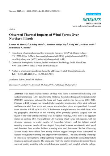
Sensors 2015, 1514985Figure 1. Geographic location of three wind farms labeled WFA, WFB, and WFC, builtbetween 2007 and 2010, together with (a) two sounding station sites (KILX and KDVN) andone Automated Surface Observing System (ASOS) station site (PNT) and (b) individual windturbines over the study region (40.86 N–41.34 N, 88.82 W–88.30 W). Plus symbolsrepresent individual wind turbines; (c) Definition of wind farm pixels (WFPs, 270 pixels inred) and nearby non-wind farm pixels (NNWFPs, 400 pixels in black) at 0.01 resolution.WFPs contain at least one wind turbine; (d) Definition of upwind wind farm pixels(UWFPs, 141 pixels in orange) and downwind wind farm pixels (DWFPs, 300 pixels inblue) at 0.01 resolution. DWFPs and UWFPs are located between WFPs and NNWFPs.Initial wind turbine existence is confirmed by built dates from the FAA records for the period2003–2013 as this database encompasses any development in the study region in Illinois. The GoogleEarth image history database is then used to confirm the existence and location of each turbine. Alsopublic records and wind farm information on each wind farm validate the total number of turbines [23].2.2. Data2.2.1. Remotely Sensed DataThis study utilizes MODIS LST and land cover products derived from instruments onboard theNASA’s Terra and Aqua satellites. Terra and Aqua were launched in 1999 and 2002, respectively.Because a full year of data for both Terra and Aqua do not exist for the years 2000–2002, the studyperiod used here begins in 2003.The MODIS 8-day LST data at 1 km resolution used are the same as described in Zhou et al. [17,18],ranging from 2003 through 2013. The 8-day LST product is the average from 2 to 8 days of daily productsto reduce the daily data gap due to the presence of clouds [24]. Each satellite provides two measurementsper day and so there are four measurements in total, approximately at local solar times of 10:30 a.m. and 22:30 p.m. for Terra (MOD11A2) and 13:30 p.m. and 1:30 a.m. for Aqua (MYD11A2).Land cover information is obtained from the MODIS land cover map (MCD12Q1) at 500 m spatialresolution. It has five different classification schemes that describe land cover properties [25]. For thisstudy, the International Geosphere Biosphere Programme (IGBP) scheme, which identifies 17 land

Sensors 2015, 1514986cover classes, is chosen. There are 11 natural vegetation classes, three non-vegetated classes, and threedeveloped and mosaiced land classes. The land cover map is derived from the combined observationsfrom Terra and Aqua. Because it is composited annually, the first year of the study period (2003) iscompared to the last year of data (2012) to detect land cover/use change over the study region. Notethat the data in 2013 is not available.2.2.2. Topography DataThe United States Geological Survey (USGS) provides global 30 arc-second elevation data(GTOPO30) at approximately 1 km spatial resolution. This digital elevation data is divided into tiles,and the West 100 and North 90 tile is used to include the study region (Figure 2a).Figure 2. (a) Surface topography (m) at 1 km spatial resolution for the study region;(b) Land cover and land use map in 2003 over the study region at 0.005 spatial resolution;(c) Spatial pattern of MODIS ANN nighttime LST ( C) climatology at 0.01 spatialresolution over the study region for the period 2003–2013. Plus symbols representindividual wind turbines.

Sensors 2015, 15149872.2.3. Meteorological DataSurface wind data at 10 m above the ground for the period 2003–2013 are obtained from anAutomated Surface Observing System (ASOS) station, located in Pontiac, Illinois (PNT), which lies32 km south of the wind farms (Figure 1a). The ASOS data is retrieved from the Iowa EnvironmentalMesonet (IEM) and provide measurements at 20-minute intervals. Here we use ASOS to provide windstatistics at a location closer to the wind farms and at a higher temporal resolution covering the Terraand Aqua measurement times than sounding data. Because the majority of turbines in the study regionstand at an 80 m hub-height, and the measurements are taken only at 10 m, there will be an increase inwind speed at the higher hub-height due to lessened impacts from near surface roughness.Note that vertical profiles of wind and temperature are useful to study ABL processes at the turbinehub-height but sounding data from weather stations can only provide measurements twice daily(00 and 12 GMT). Nevertheless, two weather stations with sounding data near the wind farms are usedand compared for quality assurance. Lincoln, Illinois (04833, KILX) lies about 145 km south of thewind farms; Davenport, Iowa (94982, KDVN) lies about 200 km west (Figure 1a). The atmosphericsounding data used in this study are retrieved from the Stratosphere-troposphere Processes And theirRole in Climate (SPARC) website. This high resolution data consists of measurements taken everysecond during the ascent of the balloon for a time period ranging from 2008 through 2011. Though thisdoes not cover the entirety of the study period, it may be sufficient to collect a climatological signatureof the atmospheric profiles during the times when the wind turbines were operating. The stationsurface elevation is 179 m for KILX and 230 m for KDVN. As the average elevation of the windturbines is 213 m, we choose the sounding data around 293 m above sea level to represents the 80 mhub-height measurements. We analyzed the seasonal variations of wind profiles, which show similarfeatures as the ASOS data but with a larger magnitude. We also analyzed the temperature profiles toexamine the seasonal variations of the strength and depth of the temperature inversion layer.2.3. Data ProcessingFor each year there are 184 LST images consisting of 46 8-day composites and four measurementsper composite from both the Terra and Aqua satellites. The MODIS 8-day LST data is combined intomonthly means and is used to create monthly anomalies by subtracting the LST climatology at everypixel. The data are then further combined into seasonal mean and anomalies in DJF (Dec-Jan-Feb),MAM (Mar-Apr-May), JJA (Jun-Jul-Aug), and SON (Sep-Oct-Nov). Annual (ANN) means andanomalies are also created. There are eleven years of LST data for the period 2003–2013. For eachseason and ANN in each year, there are four images of LST corresponding to the four acquisitiontimes of the MODIS data.The wind farm-induced LST changes are a low-frequency signal while the background LST has astrong diurnal, seasonal and interannual variability, which is a high-frequency signal. In particular, theinterannual variability is strong, especially in DJF. Hence, the two MODIS LST data for daytime( 10:30 a.m. and 13:30 p.m.) and nighttime ( 22:30 p.m. and 1:30 a.m.) are combined into onedaytime and one nighttime image in each season and in ANN for every year as done in Zhou et al. [17].This averaging should reduce data noise while minimizing high-frequency variations from daily

Sensors 2015, 1514988weather events and changes in solar heating [26] and thus make the low-frequency signal easy to bedetected [17–19,21].The MODIS LST data on a sinusoidal projection are re-projected into pixels with 0.01 resolution( 1.1 km), which is slightly coarser than the original 1 km data in order to avoid spatial gaps. Thestudy region consists of 2496 pixels (52 columns, 48 rows) covering the total of 490 wind turbines(Figure 1). Similarly, the MODIS land cover map is re-projected from the 500 m spatial resolution ofthe original data set to a 0.005 spatial resolution plot. The ASOS wind speed and directionobservations are composited into hourly means by seasons as well. The daily sounding data arecomposited into seasonal means similarly.2.4. Detection and Attribution Methods2.4.1. Definition of Four Groups of PixelsFour groups of pixels at 0.01 spatial resolution (Figure 1c,d) are defined to quantify the LSTchanges and their association with the wind turbines. We define those pixels containing at least onewind turbine as wind farm pixels (WFPs), and those non-wind-farm pixels surrounding each wind farmas nearby non-wind-farm pixels (NNWFPs). NNWFPs are selected at a distance of 2 pixels away fromWFPs. Turbulence decreases farther downwind from the rotor blades [7], and a distance of ten rotordiameters downstream is enough for the flow to recover from the turbulence caused by the rotorblades [27,28]. For example, the 1.5 MW GE wind turbines have a rotor diameter of 80 m, meaning10 rotor diameters away would be 800 m [29]. The distance used here of 2 pixels at the 0.01 resolution, is over 2 km away. Even if wakes were to extend to 15 rotor diameters [30], the distancehere is still large enough to minimize most impacts from turbulence downwind of the rotors. In total,there are 270 WFPs and 400 NNWFPs (Figure 1c). The presence of wind turbines will have an effecton their downwind pixels. We further classify the 441 pixels between WFPs and NNWFPs into twogroups: upwind wind farm pixels (UWFPs, 141 pixels) and downwind wind farm pixels (DWFPs,300 pixels) (Figure 1d). As the wind direction is primarily from south and west over the study region(see more discussion in Section 3.3.4), DWFPs contain those pixels in the east and north of WFPs, andUWFPs have those pixels in the west and south of WFPs.2.4.2. Spatial Pattern AnalysisThe average LST anomalies during the pre-turbine construction period (2003–2006) are subtractedfrom those during the post-turbine construction period (2010–2013) at the pixel level. As thebackground LST varies substantially from one year to another, we remove the regional mean LSTanomaly (one constant value) from the resulting LST anomaly image to highlight the sub-regional LSTspatial variability as detailed in Zhou et al. [17,18]. By evaluating the relative LST differencesbetween these two periods, a warming or cooling signal in LST will become apparent across the studyregion. If the geographic distribution of the LST changes is generally spatially coupled with the layoutof the wind turbines (referred to as the spatial coupling hereafter), it suggests potential impacts of thewind farms on LST.

Sensors 2015, 1514989This spatial coupling can be checked by examining the spatial distribution of LST changes versusthe layout of wind farms but is also quantified by a simple method introduced here. We rank the LSTdifferences from all of the 2496 pixels within the study region in a decreasing order and pick up thefirst 5%, 10% and 15% pixels with the largest LST anomalies (the strongest warming signal). Wecalculate the percentage of these 5%, 10% and 15% pixels falling into each of the four groups ofpixels, referred to as the spatial coupling index (SCI). If the LST changes are randomly distributedspatially, the possibility of these pixels falling into the four groups (referred to as the SCI threshold)should be 10.8% (270 pixels divided by 2496 pixels) for WFPs, 16.0% (400 pixels divided by 2496pixels) for NNWFPs, 5.6% (141 pixels divided by 2496 pixels) for UWFPs, and 12.0%(300 pixels divided by 2496 pixels) for DWFPs. The SCI value can be used to quantify the degree ofspatial coupling or downwind effect of the LST changes with the wind farms.2.4.3. Temporal Variability AnalysisThe areal mean interannual LST differences (WFPs minus NNWFPs) are examined for each seasonto assess the wind farm impacts on temperature. It is reasonable to assume that WFPs and NNWFPsshare similar background meteorological conditions and so their LST differences reflect primarilyimpacts of local land surface conditions. If the operational wind farms cause a warming effect, the LSTdifferences should exhibit positive values after the wind farms are built.We quantify the wind farm impact by calculating the areal mean LST differences (WFPs minusNNWFPs) between the post- and pre- turbine construction periods (2010–2013 minus 2003–2006).Positive values mean warmer temperatures over WFPs relative to NNWFPs, suggesting an impactfrom the operational wind turbines. It is important to note that prior to the existence of the windturbines, WFPs and NNWFPs don’t have identical temperatures due to land surface heterogeneity. Theunderlying vegetation, though similar, is not expected to have exactly the same thermal effects due tovariations in vegetation amount/cover. That is why we need to calculate the areal mean LST differencebetween the post- and pre- turbine construction period to remove the LST difference between WFPsand NNWFPs even before the turbines are built.3. Results and Discussion3.1. Spatial Patterns of Wind Farm Impacts on LSTLand surface properties largely determine the climatology of LST. The MODIS land cover map(Figure 2b) shows that most of the study area under the turbines is uniformly used for crops (green).The land cover types include grassland, shrubs, forests, and cropland. There are also small urban areas(in maroon) to the north and south of the wind farms, and natural vegetation (in orange) to the northalong the river, which can be identified easier in the local topography map (Figure 2a). Figure 2cdisplays the climatology of ANN nighttime LST for the period 2003–2013. Evidently, the spatialvariations in LST are associated with the surface topography (Figure 2a) and land cover map(Figure 2b). Several large towns show an urban heat island effect. The river and its nearby vegetationare warmer than the cropland at night because the former has higher heat capacity than the latter.Effects due to surface heterogeneity like these are minimized by using the LST anomalies (deviations

Sensors 2015, 1514990from climatological means) at pixel level, as land cover and topography do not change much from oneyear to the next.The LST shows strong interannual variability over the study region. Figure 3 illustrates the regionalmean LST anomalies at nighttime and their standard deviations (STDs) from 2003 to 2013. DJF LSTchanges substantially due to variable winter weather systems each year. MAM LST also displays muchvariability from year to year. Above average LSTs in these seasons greatly impact the ANN LST in2007 and 2012. A strong negative LST anomaly in DJF in 2011 of nearly 4.0 C below average reducedthe annual LST, even though this year was 2.0 C warmer than average in JJA. The STD is largest in DJF(2.07 C), followed by MAM (1.46 C), JJA (1.19 C), and SON (0.73 C). The high-frequency LSTvariability will mask to some extent the wind farm induced low-frequency LST signal [18,19], particularlyin the winter months (see more discussion later).Figure 3. Regional mean interannual MODIS nighttime LST anomalies ( C) over the studyregion for the four seasons (DJF, MAM, JJA, and SON) and annual mean (ANN). Standarddeviations of LST anomalies are shown.Figure 4 shows the ANN LST differences between the pre-turbine construction period (2003–2006)and the post-turbine construction period (2010–2013) at the pixel level. Consistent with the previousstudies [17,18], the positive LST anomalies are spatially coupled with the wind turbines at nighttime,but the daytime LST does not display any spatial coupling with the wind turbines. Therefore, daytimeresults are excluded from this study for the sake of brevity.

Sensors 2015, 1514991Figure 4. Annual mean MODIS LST differences ( C) between two periods (2010–2013minus 2003–2006 averages) at (a) nighttime and (b) daytime. Plus symbols representpixels with at least one wind turbine.The nighttime LST difference plots between the pre- and post- turbine construction period for eachseason are shown in Figure 5. The spatial coupling of warming with the wind turbines is evident inevery season, and this coupling is the tightest in JJA, followed by SON and MAM, and the weakest inDJF, which is consistent with the quantitative analysis using the SCI index described below. Ingeneral, the shift of the warming toward the northeast corresponds to climatological wind directionsfrom the west, southwest and south, and the magnitude of warming corresponds to the strength of windspeed at hub-height (see more discussion later). The strength of the spatial coupling is also related tothe magnitude of inter-annual variability in LST (Figure 3) associated with variable weather events:larger variability causes the widespread warming seen in MAM and DJF, while less variability in SONand JJA generally mimic the overall annual variations, which are consistent with Zhou et al. [18].

Sensors 2015, 1514992Consequently, JJA, SON, and ANN have the tightest spatial coupling of nighttime warming with thewind turbines (Figures 4 and 5).Figure 5. Seasonal mean MODIS nighttime LST differences ( C) between the pre- andpost- turbine construction period (2010–2013 minus 2003–2006 averages) in (a) DJF;(b) MAM; (c) JJA and (d) SON. Plus symbols represent pixels with at least one wind turbine.We quantify this spatial coupling by comparing the SCI values of the top 5%, 10% and 15% pixelswith the strongest warming anomalies falling into WFPs compared with the corresponding SCIthreshold (10.8%) (Table 1). It should be noted that the higher the SCI, the stronger the spatialcoupling. Evidently, SCI ranges seasonally from 25.7% to 40.3% for WFPs, significantly higher thanthe 10.8% SCI threshold, pointing to the wind farms as cause of this warming effect. Generally JJAhas the highest SCI value, followed by SON and MAM, while DJF has the smallest SCI value.Compared to the seasonal SCI statistics, ANN has the highest SCI values (36.1%–54.8%) and thus thetightest spatial coupling because it has the least high-frequency LST variations that likely mask thedetection of the wind farm-induced low-frequency warming signal.

Sensors 2015, 1514993Table 1. Seasonal variations in the percentage of the top 5%, 10% and 15% pixels with thestrongest warming anomalies falling into each group of pixels (referred to as spatialcoupling index (SCI))Number of Pixels(% of Total 9WFPs, NNWFPs, DWFPs, and UWFPs are defined in the main text and shown in Figure 1. Values in bold(rows 2–16) are larger than those that would be generated randomly (the first row).3.2. Temporal Variability of Wind Farm Impacts on LSTFigure 6 shows the areal mean seasonal and ANN time series of LST differences (WFPs minusNNWFPs) from 2003 to 2013. Despite a strong interannual variability, there is clearly a jump towardpositive values across all seasons after 2010, when all the turbines came online, suggesting that theconstruction of wind turbines warm WFPs relative to NNWFPs. We can quantify the magnitude of thewarming effect by subtracting the LST anomalies between the pre- and post-turbine constructionperiod (20

San Gorgonio Pass Wind Farm from 1984 to 2011 using higher resolution Landsat data, with a warming trend that is consistently observed downwind of the wind farm. Harris et al. [21] analyzed five wind farms in Iowa using MODIS LST data and provided further observational evidence of the wind farm-induced warming effect at nighttime.